Description of antennas
!date
mardi 29 janvier 2019, 14:28:18 (UTC+0100)
PyLayers has a rich set of tools for handling antenna radiation pattern. Antennas can be described in different manners and read from different specific file formats.
The description goes from a simple antenna gain formula to a full polarization description, compressed or not, using scalar or vector spherical harmonics decomposition.
In the following, some features of the Antenna class are
illustrated. The Antenna class is stored in the
antenna.py
module which is placed in the antprop module.
from pylayers.antprop.antenna import *
import pylayers.util.mayautil as myu
%matplotlib inline
An antenna object can not be loaded in specifying an existing antenna
file name as argument of the constructor. Lets start by loading an
antenna from a vsh3 file which correspond to a vector spherical
harmonics representation of an antenna measured in SATIMO near field
chamber.
A = Antenna('S1R1.vsh3')
The object antenna shows itself just by typing its name.
A
type : vsh3
------------------------
------------------------
file name : S1R1.vsh3
fmin : 0.80GHz
fmax : 5.95GHz
step : 50.00MHz
Nf : 104
Br
-------------
Nf   : 104
fmin (GHz) : 0.8
fmax (GHz) : 5.95
Ncoeff s3 : 72

Bi
-------------
Nf   : 104
fmin (GHz) : 0.8
fmax (GHz) : 5.95
Ncoeff s3 : 72

Cr
-------------
Nf   : 104
fmin (GHz) : 0.8
fmax (GHz) : 5.95
Ncoeff s3 : 72

Ci
-------------
Nf   : 104
fmin (GHz) : 0.8
fmax (GHz) : 5.95
Ncoeff s3 : 72
Not evaluated
We got information about the antenna filename and the frequency band where it has been defined.
At loading time the antenna is not evaluated. It means that there is not internally any instanciation of the pattern for a set of angular and frequency values.
To list all the available antenna files in the dedicated directory of
the project it is possible to invoke the ls() method.
Antenna files should be stored in the sub-directory ant of the
current project. The current project is located with the $BASENAME
environment variable.
!echo $BASENAME
/home/uguen/Bureau/P1
We can use the ls method to determine the number of files of
different type
lvsh3 = A.ls('vsh3')
lssh3 = A.ls('sh3')
lmat = A.ls('mat')
print("Number of antenna in .vsh3 format : ",len(lvsh3))
print("Number of antenna in .sh3 format : ",len(lssh3))
print(lvsh3[0:5])
print(lssh3[0:5])
print(lmat[0:5])
Number of antenna in .vsh3 format :  69
Number of antenna in .sh3 format :  100
['AaltoHorn.vsh3', 'CEA_OTA.vsh3', 'CEA_OTA_p2.vsh3', 'S1R1.vsh3', 'S1R10.vsh3']
['3GPP_AnkleLeft.sh3', '3GPP_AnkleLeft_2.sh3', '3GPP_AnkleLeft_3.sh3', '3GPP_AnkleLeft_7.sh3', '3GPP_AnkleRight.sh3']
['S1R1.mat']
As already mentionned, the radiation pattern of the antenna has not yet
been evaluated. The method to evaluate the pattern is eval() with
the grid option set to
True. If thegridoption is set toFalse`, the antenna is
evaluated for only the specified direction. This mode is used in the ray
tracing, while the former is used to visualize the whole antenna
pattern.
The vector spherical coefficients are strored in A.C. This C letter
refers to the coefficients. Those coefficients are obtained thanks to
the Spherepack
Module.
Adams, J.C., and P.N. Swarztrauber, 1997: Spherepack 2.0: A Model Development Facility. NCAR Technical Note NCAR/TN-436+STR, DOI: 10.5065/D6Z899CF.
We are here using the same notations. See Formula 4-10- to 4-13 of the
above reference document. Only the vector spherical analysis is done
using the vha function Spherepack, the vector spherical
synthesis has been numpyfied in the
pylayers.antprop.spharm.py
module.
Description of Vector Spherical Harmonics
The coefficients of the antenna also have a repr
A.C
Br
-------------
Nf   : 104
fmin (GHz) : 0.8
fmax (GHz) : 5.95
Ncoeff s3 : 72

Bi
-------------
Nf   : 104
fmin (GHz) : 0.8
fmax (GHz) : 5.95
Ncoeff s3 : 72

Cr
-------------
Nf   : 104
fmin (GHz) : 0.8
fmax (GHz) : 5.95
Ncoeff s3 : 72

Ci
-------------
Nf   : 104
fmin (GHz) : 0.8
fmax (GHz) : 5.95
Ncoeff s3 : 72
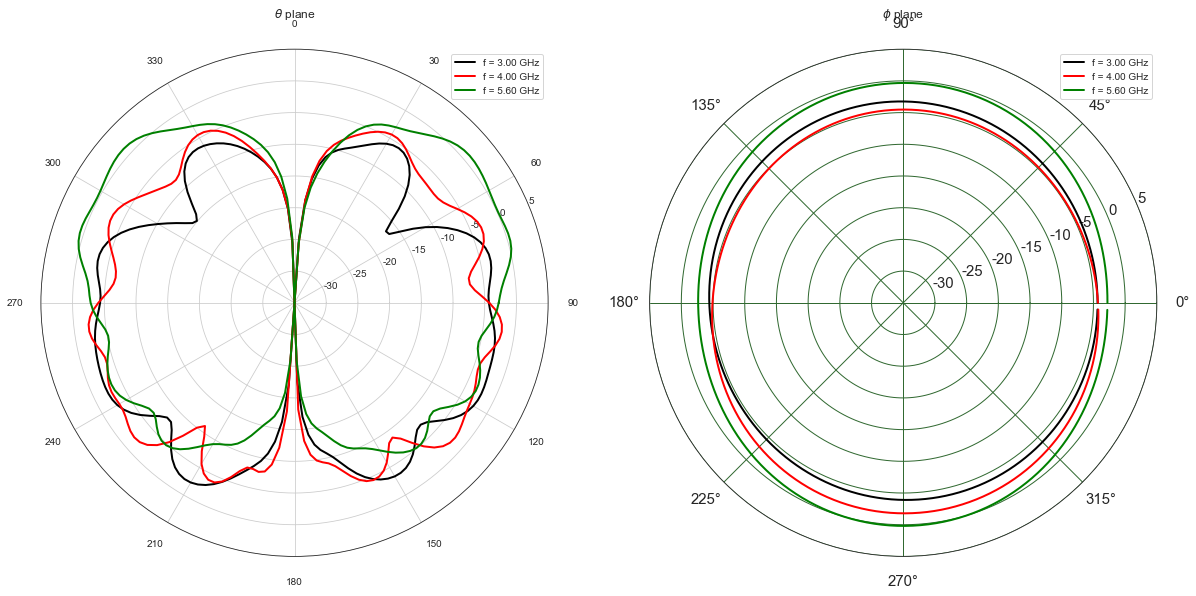
Synthesis of the radiation pattern
The radiation pattern is synthetized with the following call
A.eval(grid=True)
20*np.log10(np.max(A.sqG))
2.2267467105871743
The plotG() method allow to superpose different pattern for a list
of frequencies fGHz + If phd (phi in degree) is specified the
diagram is given as a function of \(\theta\) + If thd (theta in
degree) is specified the diagram is given as a function of \(\phi\)
f = plt.figure(figsize=(20,10))
a1 = f.add_subplot(121,projection='polar')
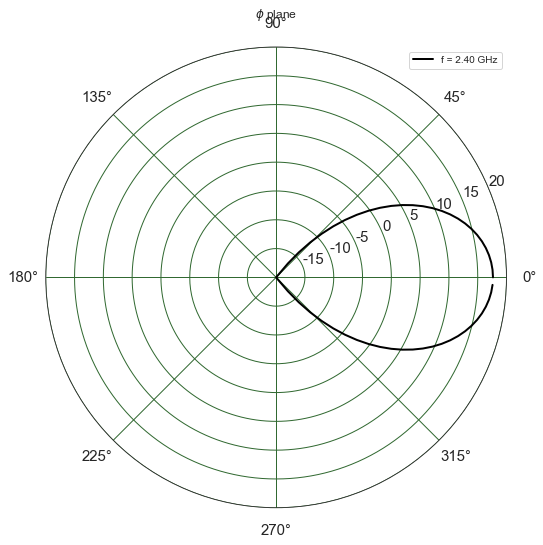
f1,a1 = A.plotG(fGHz=[3,4,5.6],plan='theta',angdeg=0,GmaxdB=5,fig=f,ax=a1,show=False)
a2 = f1.add_subplot(122,projection='polar')
f2,a2 = A.plotG(fGHz=[3,4,5.6],plan='phi',angdeg=90,GmaxdB=5,fig=f,ax=a2)
f2.tight_layout()
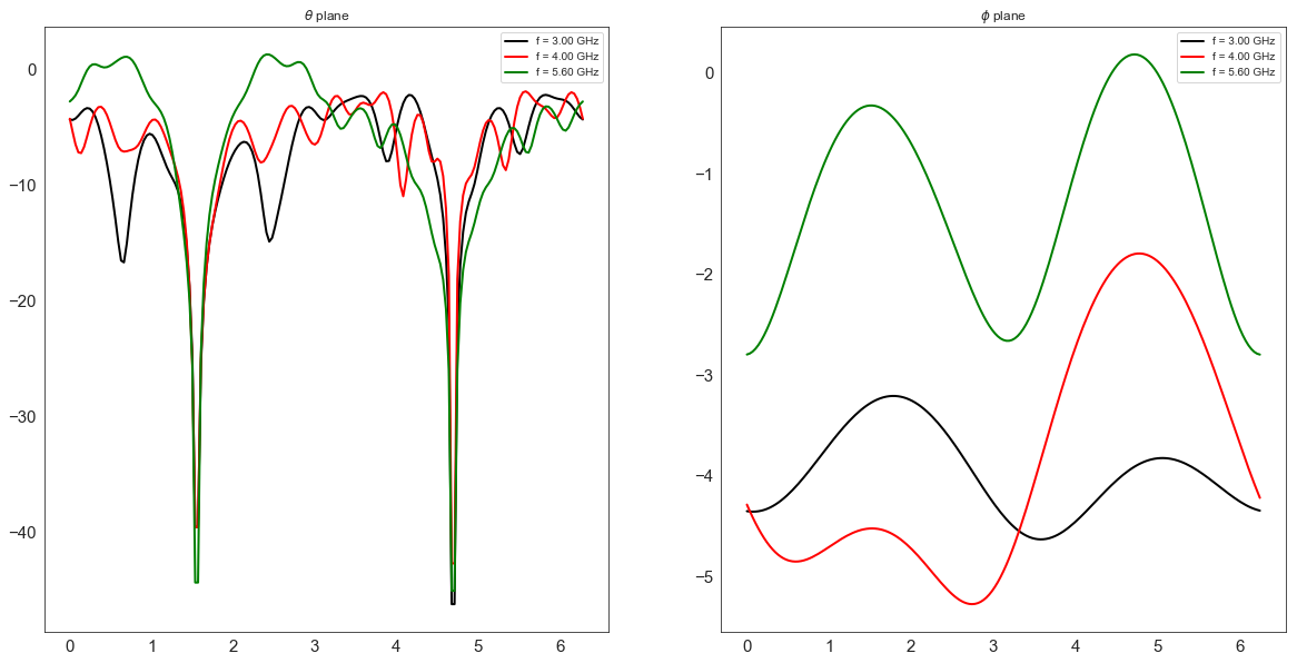
f = plt.figure(figsize=(20,10))
a1 = f.add_subplot(121)
f1,a1 = A.plotG(fGHz=[3,4,5.6],plan='theta',angdeg=0,fig=f,ax=a1,show=False,polar=False)
a2 = f.add_subplot(122)
f2,a2 = A.plotG(fGHz=[3,4,5.6],plan='phi',angdeg=90,GmaxdB=5,fig=f1,ax=a2,polar=False)
f2.tight_layout()
A.fGHz[96]
5.6000000000000005
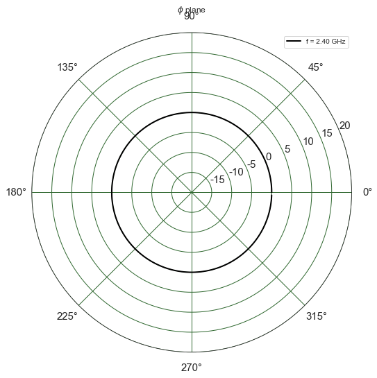
A.plotG(fGHz=[5.6],plan='phi',angdeg=90,GmaxdB=5)
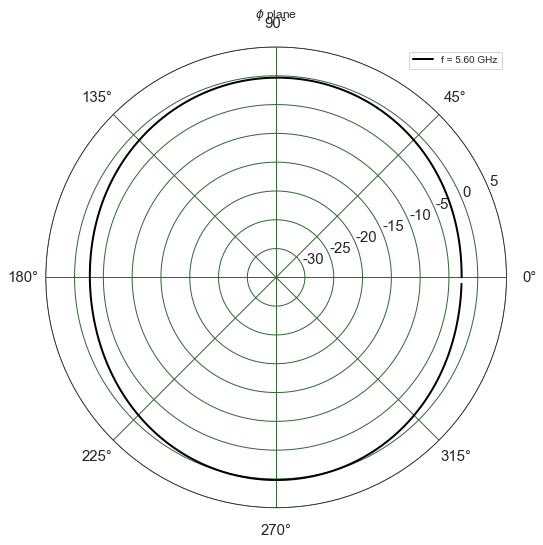
(<matplotlib.figure.Figure at 0x7fe8f574f128>,
 <matplotlib.projections.polar.PolarAxes at 0x7fe8f5759358>)
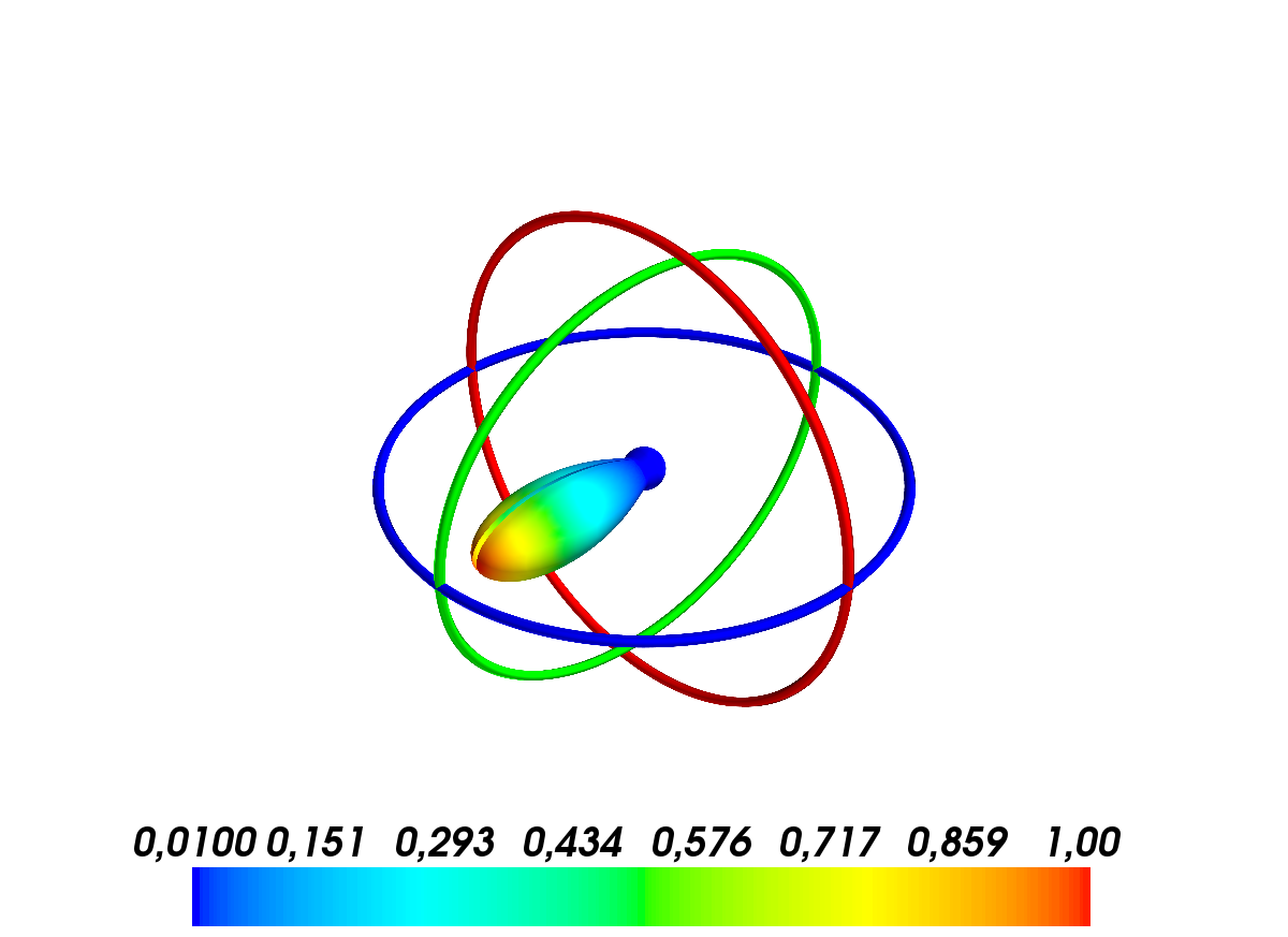
This command invoques geomview for a 3D vizualization of the radated vector field
# A.pol3d(R=5,St=8,Sp=8)
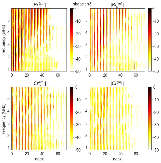
The vector spherical coefficients can be dispalayed as follows
fig = plt.figure(figsize=(8,8))
A.C.show(typ='s3')
plt.tight_layout()
Defining Antenna gain from analytic formulas
An antenna can also be defined from closed-form expressions. Available antennas are the following
Omni
Ao = Antenna('Omni')
Ao.plotG()
(<matplotlib.figure.Figure at 0x7fe8f4c81630>,
 <matplotlib.projections.polar.PolarAxes at 0x7fe8f56757f0>)
WirePlate
3GPP
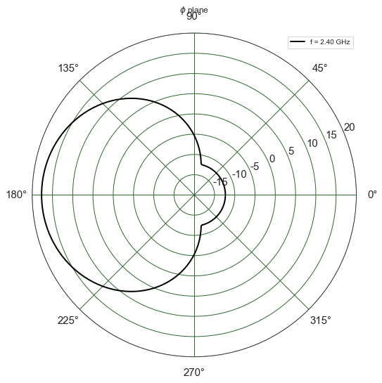
A3 = Antenna('3gpp')
A3.plotG()
(<matplotlib.figure.Figure at 0x7fe8f5262cc0>,
 <matplotlib.projections.polar.PolarAxes at 0x7fe8f4be29e8>)