Outdoor Radio Coverage with Deygout Method

This is an example of path loss prediction with Deygout method with srtm data.

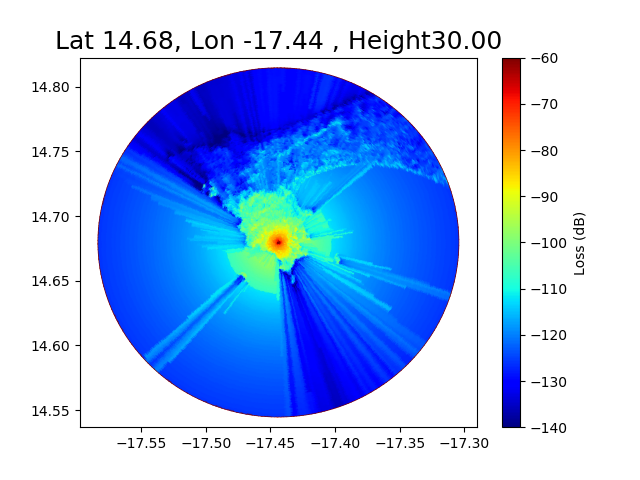
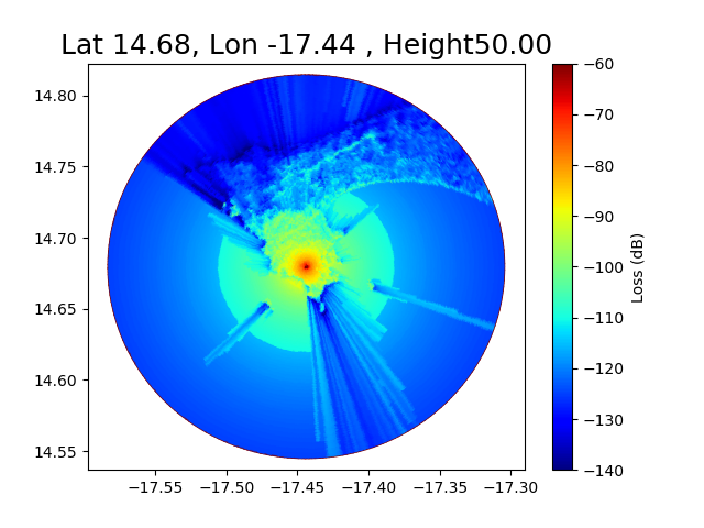
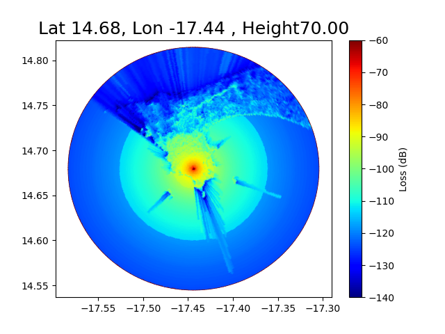
Here a comparison of the coverage for 3 different heights 30, 50, 70, meters.

f = 474.166 MHz Transmitter in Dakar (Senegal)

• 
• 
• 

Out:

SRTMDownloader - server= dds.cr.usgs.gov, directory=srtm/version2_1/SRTM3.
N14W018.hgt.zip
 Computation time : 16.84 seconds
 Computation time : 15.92 seconds
 Computation time : 15.60 seconds

from pylayers.gis.ezone import *
import pandas as pd
import matplotlib.pyplot as plt
import numpy as np
import time
#
# RTS Transmitter
#

latgw = 14.679693
longw = -17.443819
tilename = enctile(longw,latgw)
dem=DEM(enctile(longw,latgw))
dem.dwlsrtm()
xgw,ygw = dem.m(longw,latgw)
ez = Ezone(enctile(longw,latgw))
ez.hgts=dem.hgts
ez.rebase('srtm')
pa = np.array([longw,latgw])
for Ht in [30,50,70]:
    tic = time.time()
    L1 = ez.cover(pc=pa, Ht=Ht, Hr=1.5, Nr=200, Rmax=15000, method='deygout',
            source='srtm',fGHz=0.474166)
    toc = time.time()
    print(" Computation time : {:.2f} seconds".format(toc-tic))
    tc = plt.tripcolor(L1[0],-L1[1].flatten(),
                              shading='gouraud',
                              cmap='jet',
                              vmax=-60,
                              vmin=-140,
                              alpha = 1,
                              edgecolors='k',
                              linewidth=0.0)

    plt.title("Lat {:.2f}, Lon {:.2f} , Height{:.2f}".format(latgw,longw,Ht),fontsize=18)
    plt.axis('equal')
    cb = plt.colorbar()
    cb.set_label("Loss (dB)")
plt.show()