Slabs and Materials
%matplotlib inline
A slab is a set ol several layers of materials with specified thickness. Slabs are used to describe properties of the different constitutive elements of a building such as wall, windows ,…
In practice when describing a specific building, it is necessary to specify a set of different slabs with different characteristics.
The structure which gathers this set is SlabDB. If no file argument
is given, this structure is initialized with the default file:
slabDB.ini
This section demonstrates some features of the pylayers.antprop.slab
module.
from pylayers.antprop.slab import *
The Class SlabDB contains a dictionnary of all available Slabs. This
information is read in the file slabDB.ini of the current project
pointed by environment variable $BASENAME
S = SlabDB()
A SlabDB is a dictionnary, the keys are for the current file are shown below
S.keys()
['WINDOW_GLASS',
 'PLASTERBOARD_7CM',
 'WALL',
 'AIR',
 'CONCRETE_TC1_METIS',
 'CONCRETE_CEA',
 'WINDOW',
 'METALIC',
 'PLASTERBOARD_14CM',
 'brick',
 '_AIR',
 'DOOR',
 'FLOOR',
 'METAL',
 'PARTITION',
 'CONCRETE_20CM3D',
 'PLASTERBOARD_10CM',
 'WALL_TC2_METIS',
 'cement_block',
 'CEIL',
 'CONCRETE_6CM3D',
 'CONCRETE_15CM3D',
 'PLASTER_CEA',
 '3D_WINDOW_GLASS',
 'WALLS',
 'WOOD',
 'WOOD_TC1_METIS',
 'CONCRETE_7CM3D',
 'PILLAR',
 'ABSORBENT']
Defining a new Slab and a new Material
S.add('slab2',['STONE'],[0.15])
S.mat['STONE']
{'epr': (8.69999980927+0j),
 'index': 8,
 'mur': (1+0j),
 'name': 'STONE',
 'roughness': 0.0,
 'sigma': 3.0}
{'epr': (8.69999980927+0j),
 'index': 8,
 'mur': (1+0j),
 'name': 'STONE',
 'roughness': 0.0,
 'sigma': 3.0}
S['slab2']['lmatname']
['STONE']
['STONE']
S['slab2']['lthick']
[0.15]
[0.15]
fGHz= np.arange(3,5,0.01)
theta = np.arange(0,np.pi/2,0.01)
S['slab2'].ev(fGHz,theta)
fig = plt.figure(figsize=(10,10))
S['slab2'].pcolor()
A=S['slab2']
As any PyLayers object there is an help function for getting a
listing of which methods are implemented in the class.
A.help()
conv:  build lmat
ev:  evaluation of the Slab
excess_grdelay:  calculate transmission excess delay in ns
filter:  filtering waveform
help:  generic help
info:  display Slab Info
loss0:  calculate loss for theta=0 at frequency (fGHz)
losst:  Calculate loss w.r.t angle and frequency
pcolor:  display of R & T coefficients wrt frequency an angle
plotwrt:  plot R & T coefficients with respect to angle or frequency
show:  show slab Reflection and Transmission coefficient
tocolor:   convert slab properrties into a color
Information necessary to define a Slab
Each slab contains informations about its constitutive materials electromagnetic properties.
Below an example for a simple slab, constituted with a single material slab. The slab ‘WOOD’ is a layer of 4cm ‘WOOD’ material.
S['WOOD']['lmatname']
['WOOD']
thickness is expressed in meters
S['WOOD']['lthick']
[0.04]
S['WOOD']['color']
'maroon'
S['WOOD']['linewidth']
2
Multi layers Slab, using different stacks of materials can be easily defined using the two lists lmatname and lthick.
Notice the adopted convention naming lists starting with letter ‘l’ and dictionnaries starting with letter ‘d’
S['3D_WINDOW_GLASS']['lmatname']
['GLASS', 'AIR', 'GLASS']
S['3D_WINDOW_GLASS']['lthick']
[0.005, 0.005, 0.005]
For each constitutive material of a slab, their electromagnetic properties can be obtained as:
S['3D_WINDOW_GLASS']['lmat']
[{'epr': (3.79999995232+0j),
  'index': 4,
  'mur': (1+0j),
  'name': 'GLASS',
  'roughness': 0.0,
  'sigma': 0.0},
 {'epr': (1+0j),
  'index': 1,
  'mur': (1+0j),
  'name': 'AIR',
  'roughness': 0.0,
  'sigma': 0.0},
 {'epr': (3.79999995232+0j),
  'index': 4,
  'mur': (1+0j),
  'name': 'GLASS',
  'roughness': 0.0,
  'sigma': 0.0}]
Evaluation of a Slab
Each Slab can be evaluated to obtain the Transmission and Reflexion coefficients for
a given frequency range
a given incidence angle range (\(0\le\theta<\frac{\pi}{2}\))
fGHz = np.arange(3,5,0.01)
theta = np.arange(0,np.pi/2,0.01)

S['WOOD'].ev(fGHz,theta,compensate=True)
sR = np.shape(S['WOOD'].R)
print '\nHere, slab is evaluted for',sR[0],'frequency(ies)', 'and',sR[1], 'angle(s)\n'
Here, slab is evaluted for 200 frequency(ies) and 158 angle(s)
Transmission and Reflexion coefficients
Reflexion and transmission coefficient are computed for the given frequency range and theta range
ifreq=1
ithet=10
print '\nReflection coefficient @',fGHz[ifreq],'GHz and theta=',theta[ithet],':\n\n R=',S['WOOD'].R[0,0]
print '\nTransmission coefficient @',fGHz[ifreq],'GHz and theta=',theta[ithet],':\n\n T=',S['WOOD'].T[0,0],'\n'
Reflection coefficient @ 3.01 GHz and theta= 0.1 :

 R= [[-0.39396205-0.17289585j  0.00000000+0.j        ]
 [ 0.00000000+0.j          0.39396205+0.17289585j]]

Transmission coefficient @ 3.01 GHz and theta= 0.1 :

 T= [[-0.17594898-0.86927604j -0.00000000+0.j        ]
 [-0.00000000+0.j         -0.17594898-0.86927604j]]
Ploting Reflection and Transmission Coefficients
The method plotwrt can plot the different calculated coefficients
with respect to angle or frequency.
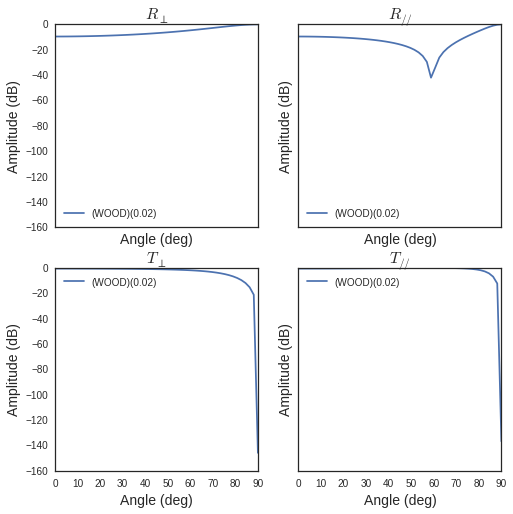
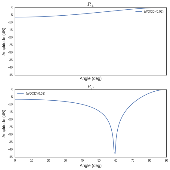
S['WOOD']['lthick']=[0.02]
S['WOOD'].ev()
S['WOOD'].ev()
f,a=S['WOOD'].plotwrt()
fGHz = np.arange(1,10,0.01)
theta = np.arange(0,np.pi/2,0.01)
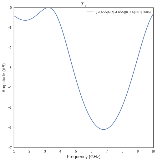
S['3D_WINDOW_GLASS']['lthick']=[0.006,0.01,0.006]
#S['3D_WINDOW_GLASS']['lmatname']=['GLASS','AIR','GLASS']
S['3D_WINDOW_GLASS'].ev(fGHz,theta)
plotwrt : plot with respect to frequency
fig,ax = S['3D_WINDOW_GLASS'].plotwrt(var='f',coeff='T',polar='o')
plot with respect to angles
fig = plt.figure(figsize=(20,20))
fGHz= np.array([2.4])
S['WOOD'].ev(fGHz,theta)
fig,ax = S['WOOD'].plotwrt(var='a',coeff='R',fig=fig)
plt.tight_layout()
<matplotlib.figure.Figure at 0x7f6a293c2d50>
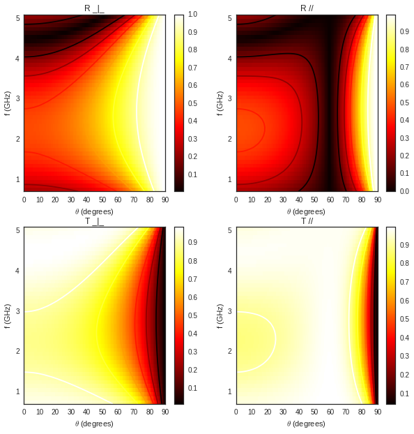
wrt to angle and frequency, use pcolor
plt.figure(figsize=(10,10))
fGHz= np.arange(0.7,5.2,0.1)
S['WOOD'].ev(fGHz,theta)
S['WOOD'].pcolor()
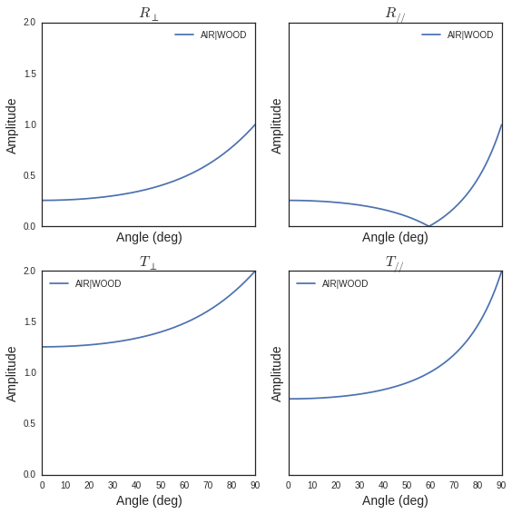
theta = np.arange(0,np.pi/2,0.01)
fGHz = np.arange(0.1,10,0.2)
sl = SlabDB('matDB.ini','slabDB.ini')
mat = sl.mat
lmat = [mat['AIR'],mat['WOOD']]
II = MatInterface(lmat,0,fGHz,theta)
II.RT()
fig,ax = II.plotwrt(var='a',kv=10,typ=['m'])
plt.tight_layout()
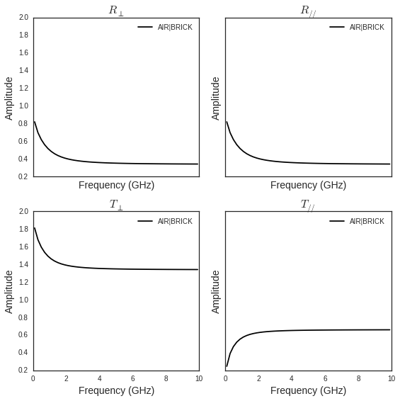
air = mat['AIR']
brick = mat['BRICK']
II = MatInterface([air,brick],0,fGHz,theta)
II.RT()
fig,ax = II.plotwrt(var='f',color='k',typ=['m'])
plt.tight_layout()
Adding new slab and materials
theta = np.arange(0,np.pi/2,0.01)
fGHz = np.arange(0.1,10,0.2)
sl = SlabDB('matDB.ini','slabDB.ini')
sl.mat.add(name='AIR2',cval=1.00000001+0j,sigma=0.00,typ='epsr')
sl.add(name='AIR-5cm',lmatname=['AIR2','AIR2'],lthick=[0.05,0.05])
sl.add(name='AIR-10cm',lmatname=['AIR2','AIR2'],lthick=[0.10,0.10])
sl.add(name='AIR-50cm',lmatname=['AIR2','AIR2'],lthick=[0.15,0.15])
fGHz=4
theta = np.arange(0,np.pi/2,0.01)
#figure(figsize=(8,8))
# These Tessereau page 50
sl['AIR-5cm'].ev(fGHz,theta,compensate=True)
sl['AIR-10cm'].ev(fGHz,theta,compensate=True)
sl['AIR-50cm'].ev(fGHz,theta,compensate=True)
# by default var='a' and kv = 0
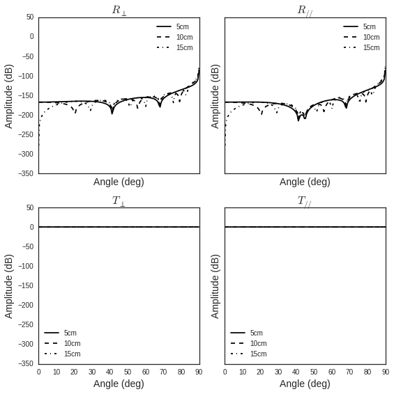
fig,ax = sl['AIR-5cm'].plotwrt(color='k',labels=['5cm'])
fig,ax = sl['AIR-10cm'].plotwrt(color='k',labels=['10cm'],linestyle='dashed',fig=fig,ax=ax)
fig,ax = sl['AIR-50cm'].plotwrt(color='k',labels=['15cm'],linestyle='dashdot',fig=fig,ax=ax)
plt.tight_layout()
Evaluation without phase compensation
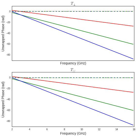
fGHz = np.arange(2,16,0.1)
theta = 0

sl['AIR-5cm'].ev(fGHz,theta,compensate=False)
sl['AIR-10cm'].ev(fGHz,theta,compensate=False)
sl['AIR-50cm'].ev(fGHz,theta,compensate=False)

fig,ax = sl['AIR-5cm'].plotwrt('f',coeff='T',typ=['ru'],labels=[''],color='r')
#print ax
fig,ax = sl['AIR-10cm'].plotwrt('f',coeff='T',typ=['ru'],labels=[''],color='g',fig=fig,ax=ax)
fig,ax = sl['AIR-50cm'].plotwrt('f',coeff='T',typ=['ru'],labels=[''],color='b',fig=fig,ax=ax)
sl['AIR-5cm'].ev(fGHz,theta,compensate=True)
sl['AIR-10cm'].ev(fGHz,theta,compensate=True)
sl['AIR-50cm'].ev(fGHz,theta,compensate=True)

# by default var='a' and kv = 0
fig,ax = sl['AIR-5cm'].plotwrt('f',coeff='T',typ=['ru'],labels=[''],color='r',linestyle='dashdot',fig=fig,ax=ax)
fig,ax = sl['AIR-10cm'].plotwrt('f',coeff='T',typ=['ru'],labels=[''],color='g',linestyle='dashed',fig=fig,ax=ax)
fig,ax = sl['AIR-50cm'].plotwrt('f',coeff='T',typ=['ru'],labels=[''],color='b',linestyle='dashdot',fig=fig,ax=ax)
plt.tight_layout()
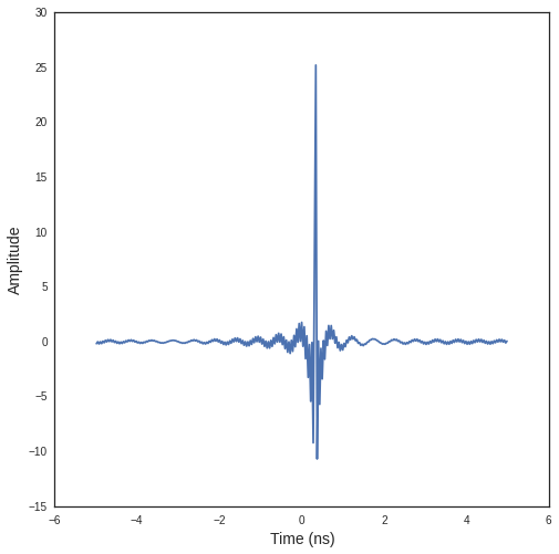
from pylayers.signal.bsignal import *
sl['AIR-5cm'].ev(fGHz,theta,compensate=False)

S = sl['AIR-5cm']
f=S.fGHz
y = S.T[:,0,0,0]
F=FUsignal(f[:,0],y)
g=F.ift(ffts=1)
g.plot(typ='v')
(<matplotlib.figure.Figure at 0x7f6a2c3b3990>,
 array([[<matplotlib.axes._subplots.AxesSubplot object at 0x7f6a2c3bd050>]], dtype=object))
sl['AIR-5cm'].ev(fGHz,theta,compensate=True)
sl['AIR-10cm'].ev(fGHz,theta,compensate=True)
sl['AIR-50cm'].ev(fGHz,theta,compensate=True)
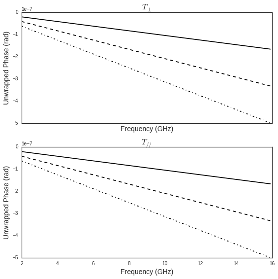
fig,ax = sl['AIR-5cm'].plotwrt('f',coeff='T',typ=['ru'],labels=[''],color='k')
#print ax
fig,ax = sl['AIR-10cm'].plotwrt('f',coeff='T',typ=['ru'],labels=[''],color='k',linestyle='dashed',fig=fig,ax=ax)
fig,ax = sl['AIR-50cm'].plotwrt('f',coeff='T',typ=['ru'],labels=[''],color='k',linestyle='dashdot',fig=fig,ax=ax)
plt.tight_layout()
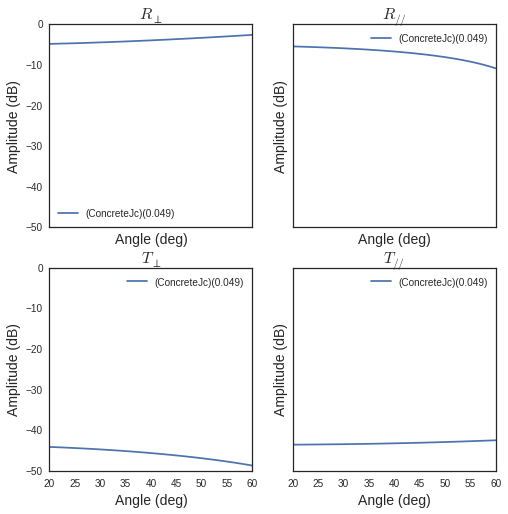
sl.mat.add(name='ConcreteJc',cval=3.5,alpha_cmm1=1.9,fGHz=120,typ='THz')
sl.mat.add(name='GlassJc',cval=2.55,alpha_cmm1=2.4,fGHz=120,typ='THz')
sl.add('ConcreteJc',['ConcreteJc'],[0.049])
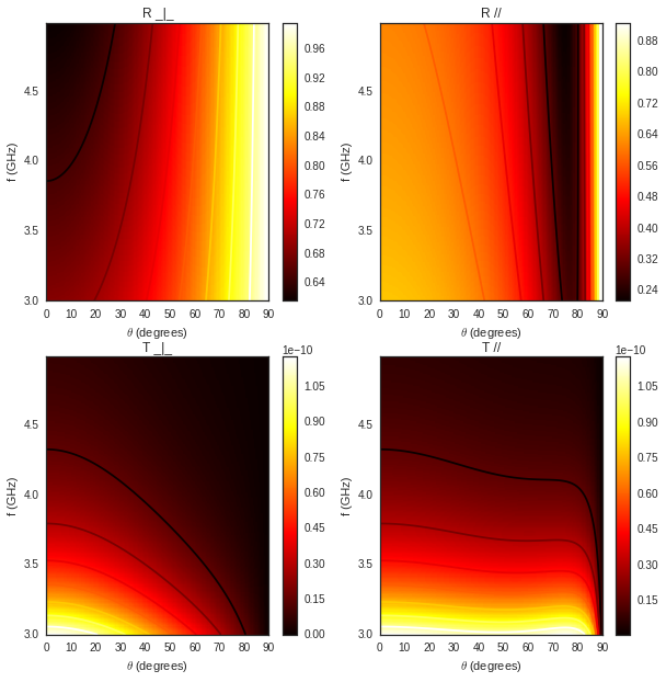
theta = np.linspace(20,60,100)*np.pi/180
sl['ConcreteJc'].ev(120,theta)
fig,ax = sl['ConcreteJc'].plotwrt('a')
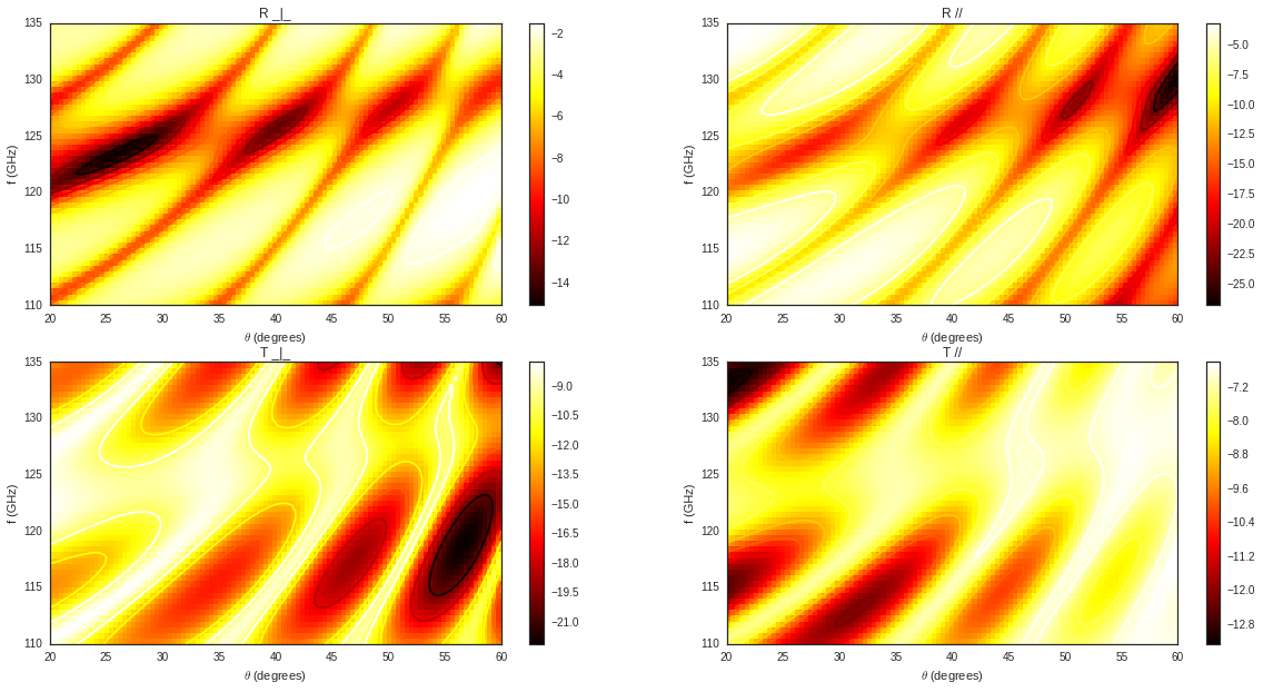
plt.figure(figsize=(20,10))
fGHz = np.linspace(110,135,50)
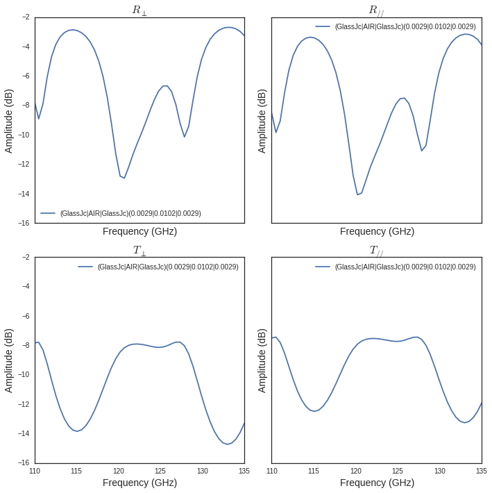
sl.add('DoubleGlass',['GlassJc','AIR','GlassJc'],[0.0029,0.0102,0.0029])
sl['DoubleGlass'].ev(fGHz,theta)
sl['DoubleGlass'].pcolor(dB=True)
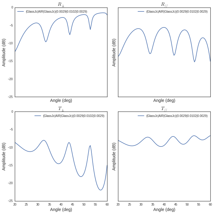
f = plt.figure(figsize=(4,4))
f = sl['DoubleGlass'].ev(120,theta)
fig,ax = sl['DoubleGlass'].plotwrt('a',figsize=(10,10))
plt.tight_layout()
<matplotlib.figure.Figure at 0x7f6a2ec701d0>
freq = np.linspace(110,135,50)
sl['DoubleGlass'].ev(freq,theta)
fig,ax = sl['DoubleGlass'].plotwrt('f',figsize=(10,10))  # @20
plt.tight_layout()