!date
vendredi 1 fvrier 2019, 08:21:12 (UTC+0100)
Description of the propagation environment
The Layout class contains the data structure for describing a
propagation environment. It contains different graphs helping the
implementation of the ray tracing. The class is implemented in the
module
layout.py
from pylayers.gis.layout import *
from IPython.display import Image
import os
%matplotlib inline
Getting the list of all available Layouts : the ls() method
Creating an empty Layout is as simple as :
L=Layout()
L
----------------
Project : /home/uguen/Bureau/P1

newfile.lay
Type : outdoor
Coordinates : cart
----------------
Gs : 0(0/0/0) :0
Gt : 0 : 0
Gr : 0 : 0
----------------


xrange : (-50, 50)
yrange : (-50, 50)
The different argument of the init function are listed below
L=Layout(arg='',
                 mat='matDB.ini',
                 slab='slabDB.ini',
                 fur='',
                 bcheck=True,
                 bbuild=True,
                 bverbose=False,
                 bcartesian=True,
             xlim=(),
                 dist_m=400,
                 typ='indoor')
string is either an existing layout filename (.lay,.osm,.res) or the coordinates (lat,lon)
mat is the a material filename material ans slab are now described in .lay file
slab is the a slab filename
fur is the furniture filename
bcheck is a boolean which force layout integrity checking
bbuild is a boolean which force rebuilding the layouts graphs
bverbose is a boolean output verbosity
bcartesian is a boolean controling the type of coordinates cartesian or (lat,lon)
xlim is a tuple with specifies the layout limits
dist_m is a float value which indicates the zone radius in meters for openstreet map extraction
typ is a string which takes values either indoor or outdoor
Querying the file name associated with the Layout.
L._filename
'newfile.lay'
The Layout is described in an .lay file, a .osmfile or a
.res file.
The ls() method lists the layout files which are available in the
struc directory of your current project, which is set up via the
$BASENAME environment variable which should be defined in order to seek
layout file in the good project directory.
L.ls('lay')
['11Dbibli.lay',
 '48.0894444444_,_-1.67388888889.lay',
 'B11.lay',
 'B11_.lay',
 'CEA.lay',
 'CEA2.lay',
 'CEA2_.lay',
 'CORM1.lay',
 'Campus_de_Beaulieu_Rennes.lay',
 'DLR.lay',
 'DLR2.lay',
 'Luebbers.lay',
 'Luebbers_v12.lay',
 'MOCAP-small.lay',
 'MOCAP-small2.lay',
 'MOCAP.lay',
 'MOCAPext.lay',
 'Munich.lay',
 'Munich_buildings.lay',
 'Rennes.lay',
 'Saint_Malo.lay',
 'Scene.lay',
 'Servon_SUr_Vilaine.lay',
 'Servon_sur_Vilaine.lay',
 'TA-Office.lay',
 'TA-Office3.lay',
 'TC1_METIS.lay',
 'TC1_METIS_2D.lay',
 'TC1_METIS_2D2.lay',
 'TC2_METIS.lay',
 'W2PTIN.lay',
 'WHERE1.lay',
 'calcul1.lay',
 'calcul2.lay',
 'defdiff.lay',
 'defsthdiff.lay',
 'defstr.lay',
 'defstr.str.lay',
 'edge.lay',
 'espoo.lay',
 'espoo2.lay',
 'espoo3.lay',
 'espoo4.lay',
 'espoo_keskus_fi.lay',
 'homeK_vf.lay',
 'klepal.lay',
 'klepal_.lay',
 'klepal__.lay',
 'lat_-1_4608251_lon_48_1218969.lay',
 'lat_12_0065911_lon_57_6954186.lay',
 'lat_48_1033333_lon_-1_61833.lay',
 'lat_48_873679_lon_2_293128.lay',
 'lat_57_696495_lon_12_006234.lay',
 'library_I2_final.lay',
 'office_I1.lay',
 'office_I1_aki_4m.lay',
 'office_I1_final.lay',
 'otakaari5A.lay',
 'otakari.lay',
 'otakari_.lay',
 'scattering.lay',
 'stromberg15GHz.lay',
 'stromberg28GHz.lay',
 'stromberg83GHz.lay',
 'test.lay',
 'test_face.lay',
 'testair0.lay',
 'testair1.lay']
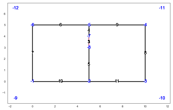
A very simple Layout which is used for testing is defstr.lay
L=Layout('defstr.lay')
L
----------------
Project : /home/uguen/Bureau/P1

defstr.lay : c9527fce60fe26328f7bacc7da6899ee
Type : indoor
Coordinates : cart
----------------
Gs : 27(12/15/3) :30
Gt : 0 : 0
Gr : 0 : 0
----------------

degree 0 : [-12 -10  -9 -11]
degree 1 : []
number of node points of degree 2 : 4
number of node points of degree 3 : 4

xrange : (-1.5, 11.5)
yrange : (-1.5, 6.5)
center : ( 5.00,2.67)
radius : 7.72
Structure of the .lay file
The description file of a Layout has the extension .lay it is an
ini file which contains the following section.
[info]
format= {cart | latlon}
version = 1.3
type = {indoor | outdoor}

[points]
-1 = (0.0,0.0)
...

[segments]
1 = {'name': ,'connect': ,'z':}
...

[slabs]
WALL = {'color: ,'linewidth': ,'lthick':[] ,'lmatname':[]}

[materials]
WOOD = {'mur':,'epr':,'sigma':,'roughness':}

[indoor] ;if type=='indoor'
zceil = 3
zfloor = 0
Layout vizualisation
The showG method is for showing the layout in specifying which graph
entities to display.
f,a=L.showG('s',
             nodes=True,
         slab=True,
         subseg=True,
         figsize=(10,10),labels=True)
Layout bounding box
L.ax provides the boundary of the layout with the following tuple format : (xmin,xmax,ymin,ymax)
L.ax
(-1.5, 11.5, -1.5, 6.5)
Layout graphs build
A Layout has to be associated with a set of graphs which are built from
the initial description in L.Gs. Those graphs are stored in pickle
files in a gpickle $BASENAME/struc/gpickle directory.
L.build()
L.Gv.node
NodeView((1, 2, 3, 4, 5, 6, 7, 8, 9, 10, 11, 17, 30, 22, -6, 27, -4, -3, -1))
A Layout is decomposed into convex cycles which are stored in the Gt
graph. The diffraction points are stored in the dictionnary L.ddiff.
The keys of this dictionnary are the diffraction points number and the
values are a zipped list of output cycles and corresponding wedge
angles.
L.ddiff
{-6: ([4, 1], 4.7123889803846897),
 -4: ([6, 4], 4.7123889803846897),
 -3: ([6, 3], 4.7123889803846897),
 -1: ([3, 1], 4.7123889803846897)}
i.e -6: ([4, 1], 4.712) means Diffracting node -6 which diffract toward the exterior sector: cycles 4 and 1 with a wedge angle of 270 degrees.
L.Gt.node
NodeView((0, 1, 2, 3, 4, 5, 6))
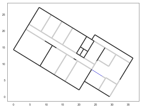
A more realistic example
Let load the DLR building
L=Layout('DLR.lay')
f,a = L.showG('s',aw=False)
To check which are the used slabs :
L.sl
List of Slabs
-----------------------------

PARTITION : |PLASTER
[0.1]
       grey80 4
       epr :(8+0j)    sigma : 0.038
CEIL : |REINFORCED_CONCRETE
[0.1]
       grey20 1
       epr :(8.69999980927+0j)    sigma : 3.0
_AIR : |AIR
[0.02]
       white 1
       epr :(1+0j)    sigma : 0.0
WALL : |BRICK
[0.07]
       grey20 3
       epr :(4.09999990463+0j)    sigma : 0.300000011921
AIR : |AIR
[0.02]
       white 1
       epr :(1+0j)    sigma : 0.0
3D_WINDOW_GLASS : |GLASS|AIR|GLASS
[0.005, 0.005, 0.005]
       blue3 1
       epr :(3.79999995232+0j)    sigma : 0.0
       epr :(1+0j)    sigma : 0.0
       epr :(3.79999995232+0j)    sigma : 0.0
FLOOR : |REINFORCED_CONCRETE
[0.1]
       grey40 1
       epr :(8.69999980927+0j)    sigma : 3.0
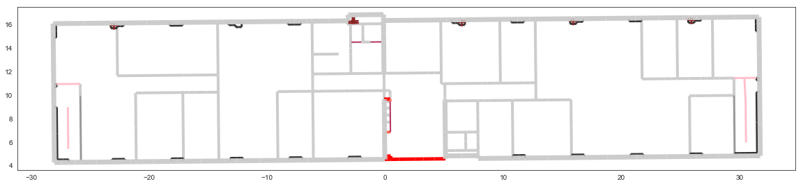
Lets load an other layout. This an indoor office where the FP7 WHERE project UWB impulse radio measuremnts have been performed.
L=Layout('WHERE1.lay')
The showG method provides many possible visualization of the layout
f,a=L.showG('s',airwalls=False,figsize=(20,10))
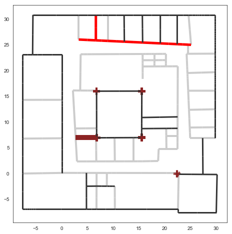
L=Layout('W2PTIN.lay')
f,a = L.showG('s')
The useful numpy arrays of the Layout
The layout data structure is a mix between graph and numpy array. numpy arrays are used when high performance is required while graph structure is convenient when dealing with different specific tasks. The tricky thing for the mind is to have to transcode between node index excluding 0 and numpy array index including 0. Below are listed various useful numpy array which are mostly used internally.
tsg : get segment index in Gs from tahe
isss : sub-segment index above Nsmax
tgs : get segment index in tahe from Gs
lsss : list of segments with sub-segment
sla : list of all slab names (Nsmax+Nss+1)
degree : degree of nodes
pt the array of points
The point coordinates are stored in two different places
L.Gs.pos : in a dictionary form (key is the point negative index)
L.pt : in a numpy array
print(np.shape(L.pt))
print(len([ x for x in L.Gs.pos.keys() if x <0]))
(2, 185)
185
This dual storage is chosen for computational efficiency reason. The
priority goes to the graph and the numpy array is calculated at the end
of the edition in the Layout.g2npy method (graph to numpy) which
handle the conversion.
tahe (tail-head)
tahe is a \((2\times N_{s})\) where \(N_s\) denotes the
number of segments. The first line is the tail index of the segment
\(k\) and the second line is the head of the segment \(k\).
Where \(k\) is the index of a given segment (starting in 0).
L.build()
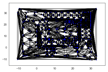
The figure below illustrates a Layout and a superimposition of the graph of cycles \(\mathcal{G}_c\). Those cycles are automatically extracted from a well defined layout. This concept of cycles is central in the ray determination algorithm which is implemented in PyLayers. Notice that the exterior region is the cycle indexed by 0. All the rooms which have a common frontier with the exterior cycle are here connected to the origin (corresponding to exterior cycle).
f,a = L.showG('s')

lp1 = nx.draw_networkx_nodes(L.Gi,L.Gi.pos,node_color='blue',node_size=1)
lp2 = nx.draw_networkx_edges(L.Gi,L.Gi.pos,node_color='blue',node_size=1)
tgs : trancodage from graph indexing to numpy array indexing
tgs is an array with length \(N_s\)+1. The index 0 is not used
because none segment has 0 as an index.
ns = 5
utahe = L.tgs[ns]
tahe = L.tahe[:,utahe]
ptail = L.pt[:,tahe[0]]
phead = L.pt[:,tahe[1]]
print(ptail)
[ 29.785 6.822]
print(phead)
[ 27.414 6.822]
L.Gs.node[5]
{'connect': [-8, -139],
 'iso': [326],
 'name': 'PARTITION',
 'ncycles': [70, 72],
 'norm': array([ 0.,  1.,  0.]),
 'offset': 0,
 'transition': False,
 'z': (0, 3.0)}
print(L.Gs.pos[-8])
(29.785, 6.822)
aseg = np.array([4,7,134])
print(np.shape(aseg))
(3,)
pt  = L.tahe[:,L.tgs[aseg]][0,:]
ph = L.tahe[:,L.tgs[aseg]][1,:]
pth = np.vstack((pt,ph))