!date

mardi 29 janvier 2019, 13:52:50 (UTC+0100)

import pylayers.gis.ezone as ez
from pylayers.gis.gisutil import ent,ext2qt
import matplotlib.pyplot as plt
import numpy as np
import seaborn as sns

%matplotlib inline

Geographical Information and the Earth Zone class : Ezone

The Ezone class handles an earth zone which corresponds to the srtm or aster DEM data. It has the same naming convention as srtm files and corresponds to a portion of earth corresponding to 1 latitude and 1 of longitude. An Ezone is an heterogeneous dataset stored in hdf5 format. Let see an example with the file N48W002.h5.

By default files are placed in directory gis/h5 of the current project tree.

The command h5ls allows to see the hierarchical structure of the file

!h5ls $BASENAME/gis/h5/N48W002.h5

bldg                     Group
dem                      Group
extent                   Dataset {4}

Invoking an earth zone requires to specify the tile prefix with the same naming convention as with SRTM files. For example let consider the earth zone from -2 to -1 in west longitude and from 48 to 49 in North latitude this corresponds to the N48W002 tile, so the ezone z is invoked as :

z = ez.Ezone('N48W002')

In this initial phase no data is loaded yet, to load all the data gathered for this Ezone in an existing HDF5 file let invoque the loadh5 method.

z.loadh5()

z

N48W002
--------
latlon (deg) : [-2 -1 48 49]
cartesian (meters) : [0.000 73676.623 0.000 111194.358 ]

Buildings
---------
i-longitude : 64 96
i-latitude  : 19 38
---------
DEM Aster (hgta) :(3601, 3601)
DEM srtm (hgts) :(1201, 1201)

This object contains the srtm DEM data, the aster data and a filtration of the open street map database selecting only the ways with building attribute. Lets have a look to the data with the show method.

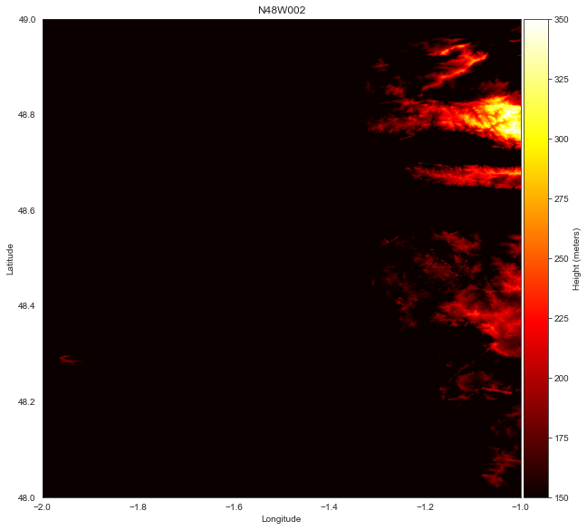
f,a,axd,md = z.show(source='srtm',bldg=False,height=True,clim=[150,350],cmap=plt.cm.hot,alpha=1)

The Ezone object has a member extent which gives [lonmin,lonmax,latmin,latmax]

z.extent

array([-2, -1, 48, 49])

The shape of hgta data is larger (3601,3601) than the srtm data (1201,1201)

z.hgta.shape

(3601, 3601)

z.hgts.shape

(1201, 1201)

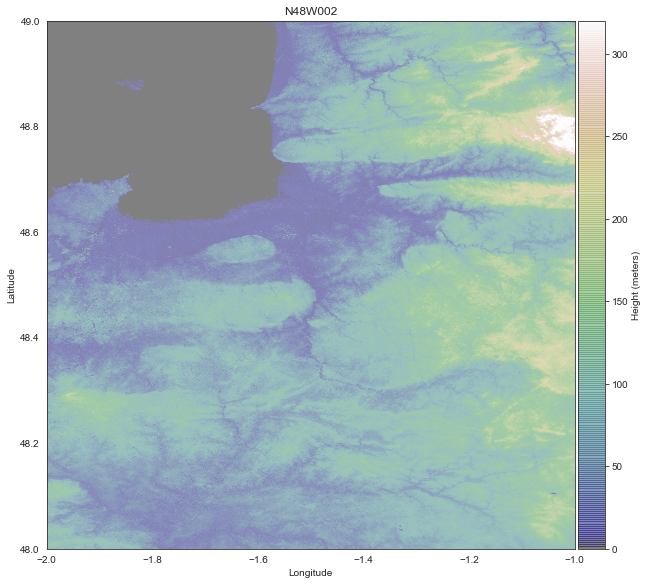
The aster DEM can also be shown.

f,a,axd,md =z.show(source='aster',bldg=False,clim=[0,320])

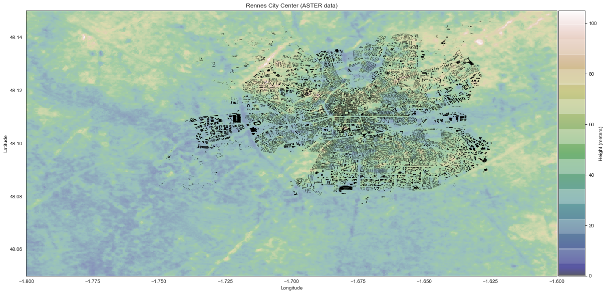
An earth zone has an attached dictionary of buildings, which contains the data of all the set of building footprints of the city extracted out of open street map data. Below is shown an example for the city of Rennes in Brittany (France).

Zooming in

For zooming into a smaller region, we define the zone to visualize a given rectangular region with (lonmin,lonmax,latmin,latmax).

This region can be converted into Cartesian coordinates with the conv method.

extent1 = (-1.8,-1.6,48.05,48.15)
extent1_cart  = ez.conv(extent1,z.m)
print("latlon extent :",extent1)
print("Cartesian extent (meters):",extent1_cart)

latlon extent : (-1.8, -1.6, 48.05, 48.15)
Cartesian extent (meters): [ 14902.21631867  29782.95775577   5482.5311488   16563.42201904]

Once the selected extent has been chosen, it is possible to pass it to the show method for zooming in the map.

f,a,axd,md = z.show(title='Rennes City Center (ASTER data)',
...              extent=extent1,
...              bldg=True,
...              height=True,
...              contour=False,
...              source='aster',
...              clim=[0,105],
...              figsize=(20,20)
...              )
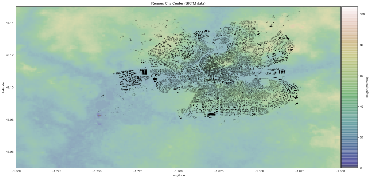
f,a,axd,md = z.show(title='Rennes City Center (SRTM data)',
...              extent=extent1,
...              bldg=True,
...              height=True,
...              contour=False,
...              source='srtm',
...              clim=[0,105],
...              figsize=(20,20)
...              )

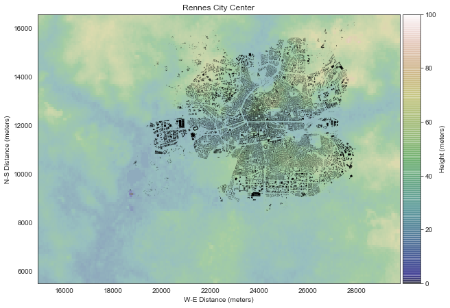
The maps diplayed above are labeled in longitude (horizontal axis) and latitude (vertical axis) but it is also possible to label it in cartesian coordinates as below

z.rebase()
z.tocart()

f,a,axd,mp = z.show(title='Rennes City Center',
...              extent=extent1_cart,coord='cartesian',
...              bldg=True,height=True,
...              clim=[0,100])

unrecognized source

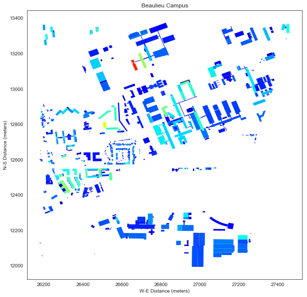
Let zoom to the University of Rennes 1 campus in the North-East region of the city.

extent2 = (-1.645,-1.62,48.111,48.125)
extent2_cart = ez.conv(extent2,z.m)
print(extent2)
print(extent2_cart)

(-1.645, -1.62, 48.111, 48.125)
[ 26436.36082369  28294.87716098  12232.14024031  13785.67272678]

f,a,axd,mp = z.show(title='Beaulieu Campus',
              extent=extent2_cart,
              coord='cartesian',
              height=False,
              bldg=True,
              clim=[0,40])

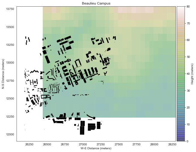
f,a,axd,mp = z.show(title='Beaulieu Campus',
              extent=extent2_cart,
              coord='cartesian',
              bldg=True,
              height=True,
              clim=[0,80])

unrecognized source

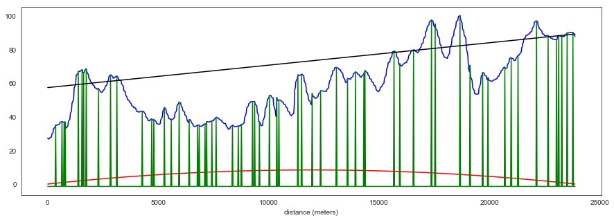
Ground Height Profile Extraction

For predicting the radio propagation, it is necessary to retrieve the height profile between 2 points on the earth surface. The profile method does a profile extraction and geometrical calculation for further propagation loss determination using the Deygout method. Points have to be expressed in (lon,lat) coordinates in WGS84 system.

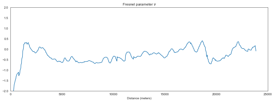
data = z.profile(pa=(-1.645,48.111),
                                 pb=(-1.62,48.325),
                                 fGHz=0.3,
                                 source='srtm')
print(data.keys())

d = : 23867.7305487
dict_keys(['ellFresnel', 'nu', 'L', 'LFS', 'height', 'hlos', 'dh', 'd', 'height_old', 'm', 'numax'])

/home/uguen/Documents/rch/devel/pylayers/pylayers/gis/ezone.py:702: RuntimeWarning: divide by zero encountered in true_divide
  fac = np.sqrt(2*d[-1]/(lmbda*d*d[::-1]))

f = plt.figure(figsize=(15,5))
d = data['d']
dh = data['dh']
h = data['height']
m = data['m']
LOS = data['hlos']
nu = data['nu']
a=plt.plot(d,dh,'r',d,h,'b',d,m[0,:],'g',d,LOS,'k')
plt.xlabel('distance (meters)')

<matplotlib.text.Text at 0x7f533c45e240>

f = plt.figure(figsize=(15,5))
a = plt.plot(d,nu)
a = plt.axis([0,25000,-2,2])
plt.title(r'Fresnel parameter $\nu$')
plt.xlabel('Distance (meters)')

<matplotlib.text.Text at 0x7f533c3e47f0>