Indoor Coverage with the PyLayers Multi Wall model¶

A Multi wall model accounts only for the attenuation along the direct path between Tx and Rx.

This approach do not provide information about delay spread or multi paths but it can nevertheless be useful in different contexts, as i.e optimization of an indoor radio network. The MultiWall approach provides a fast rough indication about the propagation losses.

A ray tracing approach is much more accurate, but also is much more time consuming and depending on the purpose, it is relevant to proceed with a simpler and faster site-specific approach as the Multiwall model.

``PyLayers`` provides a multiwall module which heavily relies on the core class ``Slab``. Notice that, the same core ``Slab`` module is used for Ray tracing and MultiWall model approaches.

Let’s see, how it works. First let’s import the coverage module. And the time module for performance evaluation.

from pylayers.antprop.coverage import *
from matplotlib.pyplot import *
%matplotlib inline
import time

Instantiate a coverage object. By defaut the TA-Office.ini layout is loaded.

The coverage information is placed in the coverage.ini file in the project directory.

Below is an example such a configuration file.

!cat $BASENAME/ini/coverage.ini

[grid]
nx = 40
ny = 20
boundary = [20,0,30,20]
mode = full ; file, zone , full
file = 'points.ini'

[layout]
filename = TA-Office.ini ; 0 40 0 15
;filename = W2PTIN.ini
;filename = Lstruc.str

[ap]
0 = {'name':'room1','wstd':'ieee80211b','p':(1,12,1.2),'PtdBm':0,'chan':[11],'on':True}
1 = {'name':'room2','wstd':'ieee80211b','p':(10,2,1.2),'PtdBm':0,'chan':[11],'on':True}
2 = {'name':'room3','wstd':'ieee80211b','p':(20,1,1.2),'PtdBm':0,'chan':[11],'on':True}
3 = {'name':'room4','wstd':'ieee80211b','p':(36.5,1.5,1.2),'PtdBm':0,'chan':[11],'on':True}
4 = {'name':'room5','wstd':'ieee80211b','p':(25,12,1.2),'PtdBm':0,'chan':[11],'on':True}

[rx]
temperaturek = 300
noisefactordb = 0

[show]
show = True

The ini file contains 5 sections.

[grid] section This section precises the size of the grid. By default the grid is placed over the whole region of the Layout. A selected region can also be defined whith the boundary list
[layout] section The name of the layout file (filename = )
[ap] section A dictionnary of access points precising the standard, the used channel, the emitted power and the position of the access point.
[show] section

# Create a Coverage object from coverag.ini file
C = Coverage('coverage.ini')

building Layout ...
check len(ncycles) == 2 passed

C has a dictionnary dap (dictionnary of access points) which gathers information about each access points of the scene.

C.dap[1]

name : room2
p : (10, 2, 1.2)
PtdBm : 0
channels  : [11]   2.462 : [2.451,2.473]
sensdBm : -94
nant : 1
On : True

The coverage object has a __repr__ method which summarizes different parameters of the current coverage object

Layout file : TA-Office.ini

-----list of Access Points ------
name : room1
p : (1, 12, 1.2)
PtdBm : 0
channels  : [11]   2.462 : [2.451,2.473]
sensdBm : -94
nant : 1
On : True

name : room2
p : (10, 2, 1.2)
PtdBm : 0
channels  : [11]   2.462 : [2.451,2.473]
sensdBm : -94
nant : 1
On : True

name : room3
p : (20, 1, 1.2)
PtdBm : 0
channels  : [11]   2.462 : [2.451,2.473]
sensdBm : -94
nant : 1
On : True

name : room4
p : (36.5, 1.5, 1.2)
PtdBm : 0
channels  : [11]   2.462 : [2.451,2.473]
sensdBm : -94
nant : 1
On : True

name : room5
p : (25, 12, 1.2)
PtdBm : 0
channels  : [11]   2.462 : [2.451,2.473]
sensdBm : -94
nant : 1
On : True

-----Rx------
temperature (K) : 300
noisefactor (dB) : 0

--- Grid ----
mode : full
nx : 40
ny : 20

C.cover()

Let display the current Layout with hidding nodes.

fig=figure(figsize=(10,5))
C.L.display['nodes']=False
C.L.display['ednodes']=False
f,a = C.show(fig=fig)

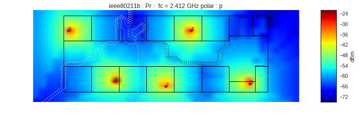
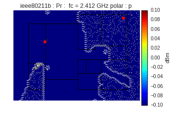
The shadowing map coverage results can be displayed by invoquing various functions.

fig=figure(figsize=(10,5))
f,a=C.show(fig=fig,typ='pr')

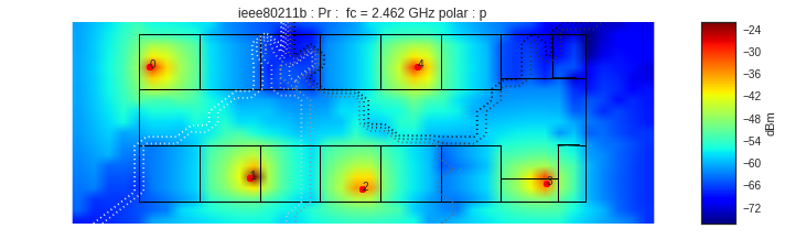
fig=figure(figsize=(10,5))
f,a=C.show(fig=fig,typ='pr',f=4)

fig=figure(figsize=(10,5))
f,a=C.show(fig=fig,typ='pr',f=10)

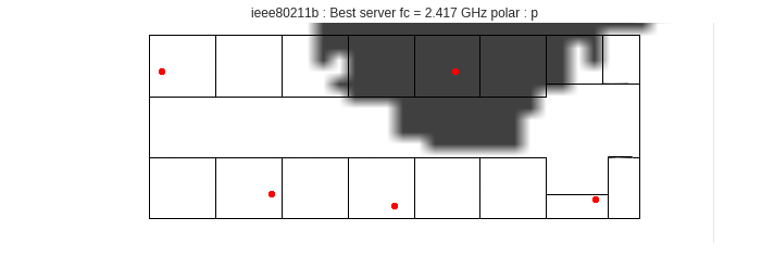
fig=figure(figsize=(10,5))
f,a=C.show(fig=fig,typ='best',f=1)

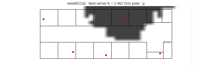
fig=figure(figsize=(10,5))
f,a=C.show(fig=fig,typ='best',f=10)

fig=figure(figsize=(10,5))
f=C.show(fig=fig,f=5,typ='sinr')

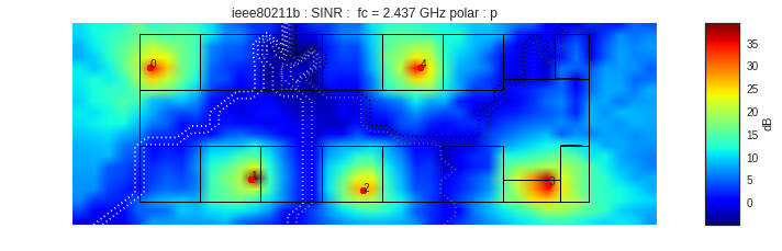
As you have noticed the calculation has been done for all the center frequencies of the selected standard. This is done in prevision of further channel optimizations.

Let’s consider an other layout

C2 = Coverage('coverage2.ini')
C2.cover()

fig=figure(figsize=(10,5))
f=C2.show(ftyp='pr')

<matplotlib.figure.Figure at 0x7fe90e684a10>

C.snro.shape

(13, 800, 5)

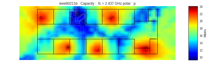
fig=figure(figsize=(10,5))
C.show(fig=fig,f=5,typ='capacity',dB=False)

(<matplotlib.figure.Figure at 0x7fe910a9d910>,
 <matplotlib.axes._subplots.AxesSubplot at 0x7fe910a9ddd0>)

All simulated quantities are stored in linear scale.

C2.Lwo[0,0,0]

0.00087507748196715026

C2.freespace[0,0,0]

1.7443256561424206e-06