Example of Utilisation of Coverage
%matplotlib inline
from pylayers.antprop.coverage import *
Load a coverage simulation file
C = Coverage('coverage2.ini')
Information about the coverage object
C
Layout file : homeK_vf.ini

-----list of Access Points ------
name : room1
p : (2.1, 6.0, 1.2)
PtdBm : 0
channels  : [11]   2.462 : [2.451,2.473]
sensdBm : -94
nant : 1
On : True

name : room2
p : (12, 9.0, 1.2)
PtdBm : 0
channels  : [11]   2.462 : [2.451,2.473]
sensdBm : -94
nant : 1
On : True

-----Rx------
temperature (K) : 300
noisefactor (dB) : 13

--- Grid ----
mode : full
nx : 50
ny : 50
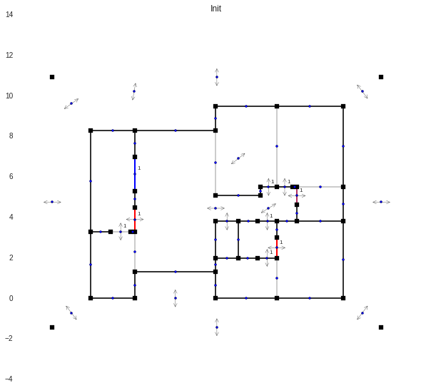
fig=plt.figure(figsize=(10,10))
f,a=C.L.showGs(fig=fig)
List of used slabs
C.L.sl
List of Slabs
-----------------------------

_AIR : AIR | [0.05]
       white 1
DOOR : WOOD | [0.05]
       red 1
FLOOR : REINFORCED_CONCRETE | [0.05]
       grey40 1
WALL : BRICK | [0.05]
       grey20 3
PARTITION : PLASTER | [0.05]
       grey80 4
METAL : METAL | [0.05]
       black 1
AIR : AIR | [0.05]
       white 1
WINDOW : WOOD | [0.05]
       blue 1
WOOD : WOOD | [0.05]
       maroon 1
CEIL : REINFORCED_CONCRETE | [0.05]
       grey20 1
ABSORBENT : AIR | [0.05]
       grey20 3
List of materials
C.L.sl.mat
List of Materials
-------------------
PLASTER (3)    |epsr|=8.00 sigma (S/m)=0.04
METAL (7)    |epsr|=1.00 sigma (S/m)=10000000.00
AIR (1)    |epsr|=1.00 sigma (S/m)=0.00
WOOD (7)    |epsr|=2.83 sigma (S/m)=3.00
BRICK (2)    |epsr|=4.10 sigma (S/m)=0.30
REINFORCED_CONCRETE (6)    |epsr|=8.70 sigma (S/m)=3.00
List associated to the slab nature of each segment.
C.L.sla
array(['', 'WALL', 'WALL', 'WALL', 'WALL', 'PARTITION', 'WALL', 'WALL',
       'WALL', 'WALL', 'WALL', 'WALL', 'WALL', 'WALL', 'PARTITION', 'WALL',
       'WALL', 'PARTITION', 'WALL', 'WALL', 'WALL', 'WALL', 'PARTITION',
       'WALL', 'WALL', 'WALL', 'WALL', 'WALL', 'WALL', 'PARTITION', 'WALL',
       'WALL', 'WALL', 'WALL', 'WALL', 'ABSORBENT', 'AIR', 'WALL', 'WALL',
       'WALL', 'WALL', 'WALL', 'WALL', 'WOOD', 'PARTITION', 'WINDOW',
       'DOOR', 'DOOR', 'WALL', 'WALL', '_AIR', '_AIR', '_AIR', '_AIR',
       '_AIR', '', '', '', '', '', '', '', '', '', '', '', '_AIR', '', '',
       '', '', '', '', '', '', '', '', '_AIR', '', '', '', '', '', '', '',
       '', '', '_AIR', '', '_AIR', '', '', '', '', '', '', '', '', '', '',
       '', '', '_AIR', '', '', '', '', '', '_AIR', '', '', '', '', '', '',
       '', '', '', '', '_AIR', 'DOOR', 'DOOR', 'DOOR', 'DOOR', 'DOOR',
       'METAL', 'AIR', 'AIR', 'AIR'],
      dtype='|S20')
Actually, calculate the coverage by invoquing the covermethod
C.cover()
fig=plt.figure(figsize=(14,8))
a1 = fig.add_subplot(121)
a2 = fig.add_subplot(122)
f,a = C.show(typ='pr',best=False,polar='o',vmin=-90,fig=fig,ax=a1)
f,a = C.show(typ='pr',best=False,polar='p',vmin=-90,fig=fig,ax=a2)

fig=plt.figure(figsize=(14,8))
a1 = fig.add_subplot(121)
a2 = fig.add_subplot(122)
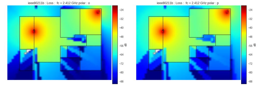
f,a = C.show(typ='loss',best=False,polar='o',vmin=-90,fig=fig,ax=a1)
f,a = C.show(typ='loss',best=False,polar='p',vmin=-90,fig=fig,ax=a2)
fig=plt.figure(figsize=(14,8))
a1 = fig.add_subplot(121)
a2 = fig.add_subplot(122)
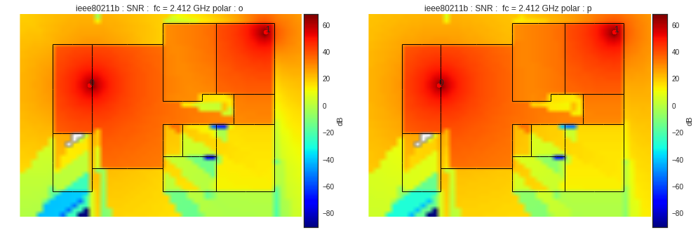
f,a = C.show(typ='snr',best=False,polar='o',vmin=-90,fig=fig,ax=a1)
f,a = C.show(typ='snr',best=False,polar='p',vmin=-90,fig=fig,ax=a2)
fig=plt.figure(figsize=(14,8))
a1 = fig.add_subplot(121)
a2 = fig.add_subplot(122)
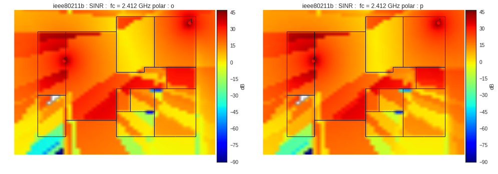
f,a = C.show(typ='sinr',best=False,polar='o',vmin=-90,fig=fig,ax=a1)
f,a = C.show(typ='sinr',best=False,polar='p',vmin=-90,fig=fig,ax=a2)
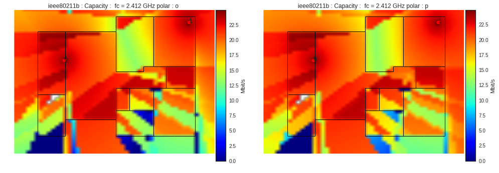
fig=plt.figure(figsize=(14,8))
a1 = fig.add_subplot(121)
a2 = fig.add_subplot(122)
f,a = C.show(typ='capacity',best=False,polar='o',vmin=0,fig=fig,ax=a1)
f,a = C.show(typ='capacity',best=False,polar='p',vmin=0,fig=fig,ax=a2)