Table Of Content
%matplotlib inline
import  pylayers.util.mayautil as myu
CORMORAN Measurement Campaign
The CORMORAN measurement campaign is the first known campaign in the WBAN context gathering :
3 differents radio technologies (HiKoB, CEA plateform and Beespoon phone)
Up to 24 radio devices equiped on a single body
A precise capture of the radio device and body movement using a Vicon motion capture (MOCAP) system.
A perfect knowledge of the capture environement
58 Series with capture or group navigation scenarios
One of the main characteristics of this measurement campaign is the use of a precise motion capture system which allows to get a ground truth position of any radio device which make the radio observable values open to insightful interpretation.
Motivation for creating a specific tool
In order to exploit the CORMORAN measurement campaign, a dedicated tool has been envisaged. Regarding that one aim of the CORMORAN project (http://pylayers.github.io/pylayers/cormoran.html) is to provide a simulation plateform from the Channel to the MAC Layer, the tool natturally takes place inside the PyLayers plateform.
This specific tool creation has been motivated by the intrinsec complexity of the the measurement campaign. First, no existing tool are able to exploit simultaneously the radio and MOCAP information from the measures.
The co-existence of 3 different radio technologies implies 3 different file formats which have to be interpreted and combined together to be exploitable. However, the motion capture, and the 3 differents radio acces technologies (RAT) operating at different sample rate, which leads to manipulating 4 different time basis. As well, no automatic start-synchronization mechanism was availble between the different technologies which leads to a non systematic time shift between the different basis.
Finally the aim of a measurement campaign is to easily provide valuable and exploitable information for the project members and more generally by people in the research community. The goal of such a tool is to help and simplify dissemination.
Prerequisite Installations
Before starting using this tool, some requirements have to be satisfied.
The open source platform PyLayers ( http://www.pylayers.org ) has to be installed following the installation notes here: https://github.com/pylayers/pylayers/blob/master/INSTALL.txt
The CORMORAN measurements have to be downloaded from the gitlab repository
An environement variable $CORMORAN has to be set at the root of your CORMORAN measurements directory (help about setup of environement variables can be found in pylayers’ INSTALL.txt
Once those 3 steps are satisfied, the CORMORAN exploitation measure tool is ready to be used.
The CorSer Class
The exploitation of measures tool takes place as a specific class named CorSer (which stands for Cormoran Series). Once PyLayers has been installed, it is possible to directly access to the class by importing it.
   from pylayers.measures.cormoran import *

Get information on the Series
Before creating the CorSer object it is possible to consult the available measurements series using cor_log(). Then for each serie of a given day it is possible to get:
The involved subject(s)
The radio technology
A short description of the serie
cor_log()
| serie | day | Subject | techno | Short Notes | |
|---|---|---|---|---|---|
| 0 | 1 | 11 | Bernard | TCR | Subject Walk circularly |
| 1 | 2 | 11 | Bernard | TCR | Subject Walk circularly |
| 2 | 3 | 11 | Bernard | TCR | Subject Walk circularly |
| 3 | 4 | 11 | Bernard | TCR | Subject Walk circularly |
| 4 | 5 | 11 | Nicolas | HKB+BS | Subject Walk circularly |
| 5 | 6 | 11 | Nicolas | HKB+BS | Subject Walk circularly |
| 6 | 7 | 11 | Nicolas | HKB+BS | Subject Walk circularly |
| 7 | 8 | 11 | Nicolas | HKB+BS | Subject Walk circularly |
| 8 | 9 | 11 | Bernard | TCR | INTERRUPTED Subject Walk circularly ++ speed |
| 9 | 10 | 11 | Bernard | TCR | Subject Walk circularly ++ speed |
| 10 | 11 | 11 | Bernard | TCR | Subject Walk circularly ++ speed |
| 11 | 12 | 11 | Bernard | TCR | Subject Walk circularly ++ speed |
| 12 | 13 | 11 | Nicolas | HKB+BS | Subject Walk circularly without looking BS pho... |
| 13 | 14 | 11 | Nicolas | HKB+BS | Subject Walk circularly + Navigation movement |
| 14 | 15 | 11 | Nicolas | HKB+BS | Subject Walk slowly without looking BS phone h... |
| 15 | 16 | 11 | Nicolas | HKB+BS | Subject Walk slowly without looking BS phone h... |
| 16 | 17 | 11 | Bernard | TCR | Static subject pointing corners then yoga post... |
| 17 | 18 | 11 | Bernard | TCR | Static subject pointing corners then yoga post... |
| 18 | 19 | 11 | Bernard | TCR | Static subject pointing corners then yoga post... |
| 19 | 20 | 11 | Bernard | TCR | Static subject pointing corners then yoga post... |
| 20 | 21 | 11 | Nicolas | HKB+BS | Static subject pointing corners (withphone) th... |
| 21 | 22 | 11 | Nicolas | HKB+BS | Static subject pointing corners (withphone) th... |
| 22 | 23 | 11 | Nicolas | HKB+BS | INTERRUPTED Static subject pointing corners (w... |
| 23 | 24 | 11 | Nicolas | HKB+BS | Static subject pointing corners (withphone) th... |
| 24 | 25 | 11 | Bernard | TCR | Kung-fu Kata |
| 25 | 26 | 11 | Bernard | TCR | Kung-fu Kata with lost sensor |
| 26 | 27 | 11 | Nicolas | HKB+BS | subject open door, sit, type on leyboard, take... |
| 27 | 28 | 11 | Nicolas | HKB+BS | subject open door, sit, type on leyboard, take... |
| 28 | 29 | 11 | Nicolas | HKB+BS | Crossfade Yoga Posture with phone BS left hand |
| 29 | 30 | 11 | Nicolas | HKB+BS | Crossfade SLOW Yoga Posture with phone BS lef... |
| 30 | 31 | 11 | Nicolas | HKB+BS | Subject Walk circularly |
| 31 | 32 | 11 | Nicolas | TCR+HKB+BS | 3 turns circularly inc. speed sequentially |
| 32 | 33 | 11 | Nicolas | TCR+HKB+BS | 3 turns circularly inc. speed sequentially |
| 33 | 34 | 11 | Nicolas | TCR+HKB+BS | 3 turns circularly inc. Speed + muscle-buildi... |
| 34 | 35 | 11 | Nicolas | TCR+HKB+BS | 3 turns circularly inc. Speed + muscle-buildi... |
| 35 | 1 | 12 | Nicolas Jihad Eric | TCR | DATA ISSUE 3 FireMen Nav |
| 36 | 2 | 12 | Nicolas Jihad Eric | TCR | 3 FireMen Nav (possible mocap issue) |
| 37 | 3 | 12 | Nicolas jihad Eric | TCR | 3 FireMen Nav (possible mocap issue) |
| 38 | 4 | 12 | Nicolas Jihad Eric | TCR | INTERRUPTED 3 FireMen Nav |
| 39 | 5 | 12 | Nicolas Jihad Eric | TCR | subjects Random walk + new interfering subject... |
| 40 | 6 | 12 | Nicolas Jihad Eric | TCR | subjects Random walk + new interfering subject... |
| 41 | 7 | 12 | Nicolas Jihad Eric | TCR | subjects slow Random walk + interfering subjec... |
| 42 | 8 | 12 | Nicolas Jihad Eric | TCR | subjects slow Random walk + interfering subjec... |
| 43 | 9 | 12 | Nicolas Jihad Eric | TCR+HKB+BS | Subject??Slow motion: Indoor Nav then Firemen t... |
| 44 | 10 | 12 | Nicolas Jihad Eric | TCR+HKB+BS | Subject??Slow motion: Indoor Nav then Firemen t... |
| 45 | 11 | 12 | Nicolas Jihad Eric | TCR+HKB+BS | Subject??normal speed: Indoor Nav then Firemen ... |
| 46 | 12 | 12 | Nicolas Jihad Eric | TCR+HKB+BS | Subject??normal speed: Indoor Nav then Firemen ... |
| 47 | 13 | 12 | Nicolas Jihad Eric | TCR+HKB+BS | subjects Random walk + new interfering subject... |
| 48 | 14 | 12 | Nicolas Jihad Eric | TCR+HKB+BS | subjects Random walk + new interfering subject... |
| 49 | 15 | 12 | Nicolas Jihad Eric | TCR+HKB+BS | subjects Random walk + new interfering subject... |
| 50 | 16 | 12 | Nicolas Jihad Eric | TCR+HKB+BS | subjects Random walk + new interfering subject... |
| 51 | 17 | 12 | Nicolas Jihad Eric | HKB+BS | NO HKB Subject??normal speed: Indoor Nav then F... |
| 52 | 18 | 12 | Nicolas Jihad Eric | HKB+BS | NO HKB Subject??normal speed: Indoor Nav then F... |
| 53 | 19 | 12 | Nicolas Jihad Eric | HKB+BS | NO HKB Subject??normal speed: Indoor Nav then F... |
| 54 | 20 | 12 | Nicolas Jihad Eric | HKB+BS | NO HKB Subject??normal speed: Indoor Nav then F... |
| 55 | 21 | 12 | Nicolas Jihad Eric | HKB+BS | subjects Random walk + new interfering subject... |
| 56 | 22 | 12 | Nicolas Jihad Eric | HKB+BS | subjects Random walk + new interfering subject... |
| 57 | 23 | 12 | Nicolas Jihad Eric | HKB+BS | subjects Random walk + new interfering subject... |
| 58 | 24 | 12 | Nicolas Jihad Eric | HKB+BS | subjects Random walk + new interfering subject... |
As an example, serie 6 from day 11 can be loaded using the following command:
S=CorSer(serie=6,day=11,layout=True)
load infrastructure node position: **** Processor coding : Intel-PC
('3GPP_omni.sh3', ' does not exist')
('3GPP_omni.sh3', ' does not exist')
('3GPP_omni.sh3', ' does not exist')
('3GPP_omni.sh3', ' does not exist')

load  Nicolas  body: **** Processor coding : Intel-PC
('3GPP_HeadRight_3.sh3', ' does not exist')
('3GPP_WristLeft_3.sh3', ' does not exist')
('3GPP_WristRight_3.sh3', ' does not exist')
('3GPP_ElbowLeft_3.sh3', ' does not exist')
('3GPP_ElbowRight_3.sh3', ' does not exist')
('3GPP_KneeLeft_3.sh3', ' does not exist')
('3GPP_AnkleLeft_3.sh3', ' does not exist')
('3GPP_AnkleRight_3.sh3', ' does not exist')
('3GPP_HipRight_3.sh3', ' does not exist')
('3GPP_BackCenter_3.sh3', ' does not exist')
('3GPP_TorsoTopLeft_3.sh3', ' does not exist')
('3GPP_TorsoTopRight_3.sh3', ' does not exist')

BS data frame index:  Align on mocap OK... time-offset applied OK

HKB data frame index: Align on mocap OK... time-offset applied OK

Create distance Dataframe... OK
/home/uguen/Documents/rch/devel/pylayers/pylayers/measures/cormoran.py:5268: FutureWarning: fill_method is deprecated to .resample()
the new syntax is .resample(...).ffill()
  df = idf.resample(str(sf)+'U',fill_method='ffill')
Once loaded information about the serie (date, type, …) can be obtained just by calling the object itself:
S
   filename : Sc20_S6_R2_HKBS
   filewear : /home/uguen/data/CORMORAN/cormoran-measures/POST-TREATED/11-06-2014/BodyandWear/Nicolas_11-06-2014_HKBS.ini
   filebody : /home/uguen/data/CORMORAN/cormoran-measures/POST-TREATED/11-06-2014/BodyandWear/Nicolas.ini
   filemocap : /home/uguen/data/CORMORAN/cormoran-measures/RAW/11-06-2014/MOCAP/serie_006.c3d
   Day : 11/06/2014
   Serie : 6
   Scenario : 20
   Run : 2
   Type : HKBS
   Original Video Id : Single
   Subject(s) : Nicolas

   Body available: True

   BeSPoon : Sc20_S6_R2_HKBS.csv
   HIKOB : Sc2_0_S6_r2_HKB_Single.mat
   ----------------------

   VC file :[6]
   Scenario :['2.0']
   Meas Serie :[6]
   Meas Run :[2]
   Subject :['Nicolas']
   techno :['HKB+BS']
   video file :[ nan]
   photo file :['100-0040']
   Radio file :['SC2.0_S6_R2_HKB_single']
   Date :['11/06/14']
   Start time :['16:12']
   Short Notes :['Subject Walk circularly']
   notes pendant mesures :['mxc3xaame chose ras ']


Available data
Radio DataFrames
Data frames are Pandas objects which can be interpreted as tables.
Each line correspond a given timestamp
Each column correspond to a given link between 2 radio devices
Depending on available RAT involved in the serie, different data frames are available:
HiKoB (HKB) data : S.hkb
BeSpoon data : S.bespo
TCR data : S.tcr
In the example serie chosen, only HiKoB and Bespoon are available.
Here is an example of the RSS values obtained by the HKB sensors for the 120 available links and the 5 first available timestamp :
S.hkb.head(5)
| AP1-AP2 | AP1-AP3 | AP1-AP4 | AP1-HeadRight | AP1-TorsoTopRight | AP1-TorsoTopLeft | AP1-BackCenter | AP1-ElbowRight | AP1-ElbowLeft | AP1-HipRight | ... | WristRight-WristLeft | WristRight-KneeLeft | WristRight-AnkleLeft | WristRight-AnkleRight | WristLeft-KneeLeft | WristLeft-AnkleLeft | WristLeft-AnkleRight | KneeLeft-AnkleLeft | KneeLeft-AnkleRight | AnkleLeft-AnkleRight | |
|---|---|---|---|---|---|---|---|---|---|---|---|---|---|---|---|---|---|---|---|---|---|
| 0.00 | NaN | NaN | NaN | NaN | NaN | NaN | NaN | NaN | NaN | NaN | ... | NaN | NaN | NaN | NaN | NaN | NaN | NaN | NaN | NaN | NaN |
| 0.01 | NaN | NaN | NaN | NaN | NaN | NaN | NaN | NaN | NaN | NaN | ... | NaN | NaN | NaN | NaN | NaN | NaN | NaN | NaN | NaN | NaN |
| 0.02 | NaN | NaN | NaN | NaN | NaN | NaN | NaN | NaN | NaN | NaN | ... | NaN | NaN | NaN | NaN | NaN | NaN | NaN | NaN | NaN | NaN |
| 0.03 | -60.0 | -64.0 | -61.0 | -71.0 | -81.0 | -73.0 | -78.0 | -79.0 | -84.0 | -73.0 | ... | -64.0 | -88.0 | -64.0 | -55.0 | -63.0 | -61.0 | -77.0 | -60.0 | -84.0 | -79.0 |
| 0.04 | -60.0 | -64.0 | -61.0 | -71.0 | -81.0 | -73.0 | -78.0 | -79.0 | -84.0 | -73.0 | ... | -64.0 | -88.0 | -64.0 | -55.0 | -63.0 | -61.0 | -77.0 | -60.0 | -84.0 | -79.0 |
5 rows ?? 120 columns
Extra data frames are also available to acces to non radio information. In particular, it exists :
S.devdf: the device dataframe, which gives mechanical information: position (x,y,z), velocity (v,vx,vy,vz) and acceleration (a,ax,ay,az) of the devices at any time stamps
S.distdf: the distance data frame, which gives ground truth distances between the different radio links.
Here is the 5 last data of the device data frame…
S.devdf.tail(5)
| id | subject | x | y | z | v | vx | vy | vz | a | ax | ay | az | |
|---|---|---|---|---|---|---|---|---|---|---|---|---|---|
| 104.19 | HKB:14 | Nicolas | 0.158588 | -1.574102 | 0.526740 | 0.012376 | -0.005046 | 0.010522 | 0.004120 | 2.242279 | 1.973267 | 0.738525 | 0.767212 |
| 104.19 | HKB:1 | 0.018552 | -2.749937 | 0.979166 | 0.000000 | 0.000000 | 0.000000 | 0.000000 | 0.000000 | 0.000000 | 0.000000 | 0.000000 | |
| 104.19 | HKB:16 | Nicolas | -0.229677 | -1.445404 | 0.175125 | 0.010564 | -0.007414 | -0.006641 | -0.003540 | 0.547866 | 0.122223 | -0.250244 | -0.471802 |
| 104.19 | HKB:10 | Nicolas | 0.262695 | -1.433168 | 1.143153 | 0.057834 | -0.048334 | -0.030042 | -0.010303 | 0.924481 | -0.697327 | 0.368652 | -0.482178 |
| 104.19 | HKB:3 | 0.021135 | 3.375590 | 1.003871 | 0.000000 | 0.000000 | 0.000000 | 0.000000 | 0.000000 | 0.000000 | 0.000000 | 0.000000 |
… and the 5 last data of the distance data frame:
S.distdf.tail(5)
| HKB:1-HKB:2 | HKB:1-HKB:3 | HKB:1-HKB:4 | HKB:1-HKB:5 | HKB:1-HKB:6 | HKB:1-HKB:7 | HKB:1-HKB:8 | HKB:1-HKB:9 | HKB:1-HKB:10 | HKB:1-HKB:11 | ... | HKB:12-HKB:15 | HKB:12-HKB:16 | HKB:13-HKB:14 | HKB:13-HKB:15 | HKB:13-HKB:16 | HKB:14-HKB:15 | HKB:14-HKB:16 | HKB:15-HKB:16 | BS:0-BS:74 | BS:0-BS:157 | |
|---|---|---|---|---|---|---|---|---|---|---|---|---|---|---|---|---|---|---|---|---|---|
| 104.15 | 6.102589 | 6.125578 | 6.135849 | 1.308815 | 1.163639 | 1.131707 | 1.387571 | 1.322510 | 1.350930 | 1.223406 | ... | 1.071233 | 0.990922 | 0.411064 | 0.753501 | 0.910143 | 0.364396 | 0.539795 | 0.445009 | 1.046829 | 0.119864 |
| 104.16 | 6.102589 | 6.125578 | 6.135849 | 1.309074 | 1.163713 | 1.131587 | 1.387549 | 1.322884 | 1.350486 | 1.223658 | ... | 1.071489 | 0.990873 | 0.410944 | 0.753502 | 0.909901 | 0.364396 | 0.539682 | 0.445027 | 1.046903 | 0.119868 |
| 104.17 | 6.102589 | 6.125578 | 6.135849 | 1.309470 | 1.163938 | 1.131414 | 1.387530 | 1.323230 | 1.350018 | 1.223874 | ... | 1.071624 | 0.990832 | 0.410933 | 0.753522 | 0.909759 | 0.364316 | 0.539533 | 0.445038 | 1.046936 | 0.119734 |
| 104.18 | 6.102589 | 6.125578 | 6.135849 | 1.309873 | 1.164064 | 1.131319 | 1.387509 | 1.323601 | 1.349608 | 1.224129 | ... | 1.071955 | 0.990734 | 0.410871 | 0.753529 | 0.909520 | 0.364281 | 0.539368 | 0.445063 | 1.047000 | 0.119982 |
| 104.19 | 6.102589 | 6.125578 | 6.135849 | 1.310357 | 1.164289 | 1.131228 | 1.387509 | 1.323915 | 1.349214 | 1.224341 | ... | 1.072294 | 0.990736 | 0.410651 | 0.753482 | 0.909291 | 0.364271 | 0.539394 | 0.445110 | 1.046967 | 0.119830 |
5 rows ?? 122 columns
The S.dev command allows to obtain the complete list of devices involved in the serie and:
the Name of the device used in the radio dataframe
the Real device Id used during the measurement campaign
The corresponding device Id used on the Body wear description
At wich Subject the device is related.
Infrastrucure access point obviously don’t have related Subject.
S.dev
   Name in Dataframe     | Real Id | Body Id  | Subject
   ========================================================
   AP4                   |       4 | HKB:4    |
   AP1                   |       1 | HKB:1    |
   AP2                   |       2 | HKB:2    |
   AP3                   |       3 | HKB:3    |
   --------------------------------------------------------
   AnkleRight            |      16 | HKB:16   | Nicolas
   KneeLeft              |      14 | HKB:14   | Nicolas
   AnkleLeft             |      15 | HKB:15   | Nicolas
   WristRight            |      12 | HKB:12   | Nicolas
   WristLeft             |      13 | HKB:13   | Nicolas
   ElbowLeft             |      10 | HKB:10   | Nicolas
   HipRight              |      11 | HKB:11   | Nicolas
   HeadRight             |       5 | HKB:5    | Nicolas
   TorsoTopRight         |       6 | HKB:6    | Nicolas
   TorsoTopLeft          |       7 | HKB:7    | Nicolas
   BackCenter            |       8 | HKB:8    | Nicolas
   ElbowRight            |       9 | HKB:9    | Nicolas
                         |         |          |
   WristRight            |     157 | BS:157   | Nicolas
   AnkleRight            |      74 | BS:74    | Nicolas
   HandRight             |       0 | BS:0     | Nicolas
   --------------------------------------------------------


Accessing the data
In order to help people not familiar with the Pandas query format, some useful methods are provided in order to extract values from radio and non radio dataframes.
### Get device position (S.getdevp)
The value of the device position at a specific time or range or time can be obtained by specifying:
The device (Name in dataframe OR real id OR body id)
The radio techno (Precising the techno is optional except when an ambiguity occurs, therefore error is raised)
a given time in second or a [start time,stop time]. If no time is given, the position for all time stamps are provided
Hence, It is possible to get the positions of the HKB radio node 11 (Hip Right), between 5.0 seconds and 5.2 seconds with:
Positions = S.getdevp(11,t=[5,5.2])
Positions
| x | y | z | |
|---|---|---|---|
| 5.00 | -0.139566 | 0.224905 | 1.016796 |
| 5.01 | -0.139553 | 0.224845 | 1.016826 |
| 5.02 | -0.139545 | 0.224825 | 1.016818 |
| 5.03 | -0.139564 | 0.224730 | 1.016849 |
| 5.04 | -0.139609 | 0.224642 | 1.016859 |
| 5.05 | -0.139580 | 0.224613 | 1.016898 |
| 5.06 | -0.139554 | 0.224586 | 1.016920 |
| 5.07 | -0.139604 | 0.224492 | 1.016937 |
| 5.08 | -0.139545 | 0.224452 | 1.016989 |
| 5.09 | -0.139521 | 0.224391 | 1.016992 |
| 5.10 | -0.139386 | 0.224397 | 1.016997 |
| 5.11 | -0.139296 | 0.224315 | 1.017041 |
| 5.12 | -0.139164 | 0.224189 | 1.017098 |
| 5.13 | -0.138988 | 0.224128 | 1.017131 |
| 5.14 | -0.138810 | 0.224048 | 1.017142 |
| 5.15 | -0.138605 | 0.223969 | 1.017148 |
| 5.16 | -0.138406 | 0.223877 | 1.017164 |
| 5.17 | -0.138043 | 0.223803 | 1.017230 |
| 5.18 | -0.137791 | 0.223654 | 1.017305 |
| 5.19 | -0.137388 | 0.223580 | 1.017321 |
| 5.20 | -0.137016 | 0.223465 | 1.017342 |
NOTE : You may also obtain a classical numpy array instead of this Pandas object by using the “*values*” method :
Positions.values
   array([[-0.13956557,  0.22490462,  1.01679608],
          [-0.13955284,  0.22484492,  1.01682581],
          [-0.13954524,  0.22482529,  1.01681787],
          [-0.1395645 ,  0.2247298 ,  1.01684918],
          [-0.13960907,  0.224642  ,  1.01685901],
          [-0.13957962,  0.2246127 ,  1.01689801],
          [-0.13955351,  0.22458575,  1.01691986],
          [-0.13960399,  0.22449205,  1.01693719],
          [-0.13954485,  0.22445244,  1.01698865],
          [-0.13952087,  0.22439058,  1.0169917 ],
          [-0.13938625,  0.22439655,  1.0169975 ],
          [-0.13929645,  0.22431535,  1.01704102],
          [-0.13916449,  0.22418907,  1.0170979 ],
          [-0.1389884 ,  0.22412761,  1.01713135],
          [-0.13880983,  0.22404759,  1.0171424 ],
          [-0.13860497,  0.22396939,  1.01714777],
          [-0.1384055 ,  0.22387668,  1.01716443],
          [-0.13804305,  0.22380293,  1.01722955],
          [-0.13779123,  0.2236543 ,  1.01730511],
          [-0.13738791,  0.22358025,  1.01732141],
          [-0.13701614,  0.22346536,  1.01734192]])


Get link value (S.getlink)
The value of a link a and b at a specific time or range or time can be obtained by specifying:
The device \(a\) (Name in dataframe OR real id OR body id)
The device \(b\) (Name in dataframe OR real id OR body id)
The radio technoa and technob (Precising the techno is optional except when an ambiguity occurs, therefore error is raised)
a given time in second or a [start time,stop time]. If no time is given, the position for all time stamps are provided
Hence, It is possible to get the HKB values between radio node 11 (Hip Right) and node 16 (Ankle Right) , between 5 seconds and 5.2 seconds with:
   Values = S.getlink(11,16,t=[5,5.2])

Get link distance (*S.getlinkd*)
The ground truth distance separating a device a and device b at a specific time or range or time can be obtained by specifying:
The device \(a\) (Name in dataframe OR real id OR body id)
The device \(b\) (Name in dataframe OR real id OR body id)
The radio technoa and technob (Precising the techno is optional except when an ambiguity occurs, therefore error is raised)
a given time in second or a [start time,stop time]. If no time is given, the position for all time stamps are provided
Hence, It is possible to get the HKB values between radio node 11 (Hip Right) and node 16 (Ankle Right) , between 5 seconds and 5.2 seconds with:
   Distances = S.getlinkd(11,16,t=[5,5.2])

Visualizing the Data
Native Pandas Vizualization
Because radio data in CorSer are stored into Pandas objects, convenient vizualization method are directly available. Most of them can be found here : http://pandas.pydata.org/pandas-docs/stable/visualization.html
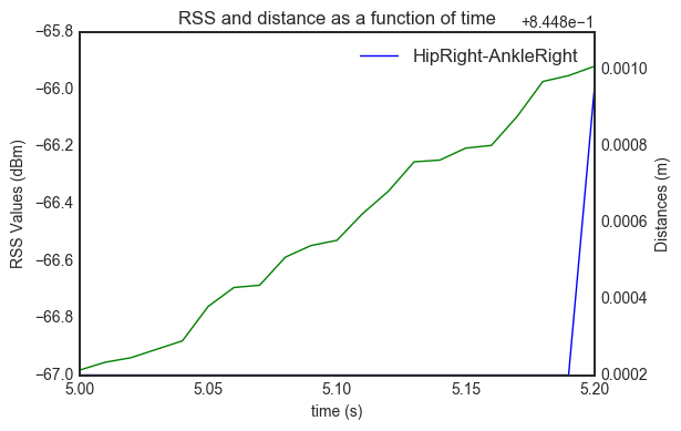
As an example, it is possible to plot the previous obtained values and distance with :
# Ploting
ax=Values.plot() #plot values
l=Distances.plot(secondary_y=True,ax=ax) # plot distances on the right side

##Labelling
ax.legend() # add legend box
ax.set_ylabel('RSS Values (dBm)') #set left ylabel
ax.right_ax.set_ylabel('Distances (m)') #set right ylabel
ax.set_xlabel('time (s)') # set xlabel
ax.set_title('RSS and distance as a function of time')
<matplotlib.text.Text at 0x7f04e8acea50>
In addition, CorSer also provides specific plotting methods which includes extra features.
Plot method (S.plot)
The plot function allows to display the radio values of a link. The main parameters are always the same:
The device \(a\) (Name in dataframe OR real id OR body id)
The device \(b\) (Name in dataframe OR real id OR body id)
The radio techno (Precising the techno is optional except when an ambiguity occurs, therefore error is raised)
A given time in second or a [start time,stop time]. If no time is given, the position for all time stamps are provided
More option are availble, please refer to the docstring (S.plot?) for more information
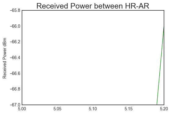
Plot values
Continuying with the same example, it is possible to plot the HKB values between radio node 11 (Hip Right) and node 16 (Ankle Right) , between 5 seconds and 5.2 seconds with:
S.plot(11,16,t=[5,5.2])
(<matplotlib.figure.Figure at 0x7f04e8b56f90>,
 <matplotlib.axes._subplots.AxesSubplot at 0x7f04e8b6b450>)
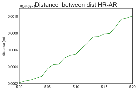
Plot distance
As well, it is possible to plot the distance using the distance parameter
S.plot(11,16,t=[5,5.2],distance = True)
(<matplotlib.figure.Figure at 0x7f04e8931350>,
 <matplotlib.axes._subplots.AxesSubplot at 0x7f04e8946050>)
It is also possible to get the same result than with the Pandas procedure with the following code :
#plot value
f,ax = S.plot(11,16,t=[5,5.2],color ='b',title=False)

# create right axis
ax2=ax.twinx()

# plot distance
S.plot(11,16,t=[5,5.2],color ='g',title=False,
        distance=True,
        fig=f,ax=ax2)
(<matplotlib.figure.Figure at 0x7f04e88d9890>,
 <matplotlib.axes._subplots.AxesSubplot at 0x7f04e8770c50>)
In order to go further in the radio value interpretation, it is convenient to have some extra information about the optical visibility/occultation of devices involved in a link.
This information allows to determine the line of sight (LOS) or non line of sight (NLOS) cases which are crutial for power level and delay interpretation.
This information can be superimposed to the radio values. To this end, the plot visibility (S.pltvisi) method is used. The hatched area denoted NLOS wheras clear area denotes LOS.
Parameters are the same than those the plot method:
f,ax = S.plot(1,16)
S.pltvisi(1,16,fig=f,ax=ax)
/home/uguen/Documents/rch/devel/pylayers/pylayers/mobility/ban/body.py:2516: VisibleDeprecationWarning: using a non-integer number instead of an integer will result in an error in the future
  C = self.d[:,kta,frameId]
/home/uguen/Documents/rch/devel/pylayers/pylayers/mobility/ban/body.py:2517: VisibleDeprecationWarning: using a non-integer number instead of an integer will result in an error in the future
  D = self.d[:,khe,frameId]
(<matplotlib.figure.Figure at 0x7f04e88e4090>,
 <matplotlib.axes._subplots.AxesSubplot at 0x7f04e88788d0>)
As well it is possible to determine and indicate whether the subject is static or not by using the plot mobility method (S.pltmob). The succession of Static and Mobile sequences are denoted \(S_x\) and \(M_x\) resplectively, where \(x\) is an index of the sequence.
f,ax = S.plot(1,16)
S.pltmob(fig=f,ax=ax)
(<matplotlib.figure.Figure at 0x7f04e8583750>,
 <matplotlib.axes._subplots.AxesSubplot at 0x7f04e8594790>)
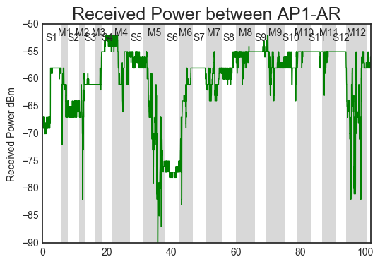
The 2 upmentionned methods can also be used simultaneously as shown in the following example :
# plot data in green)
f,ax=S.plthkb(1,13,figsize=(10,5))
# plot optical occultation (hatched lines)
S.pltvisi(1,13,fig=f,ax=ax)
# plot subject mobility (grey areas)
S.pltmob(showvel=False,ylim=([-100,-40]),fig=f,ax=ax)
(<matplotlib.figure.Figure at 0x7f04e85f2790>,
 <matplotlib.axes._subplots.AxesSubplot at 0x7f04e858b4d0>)
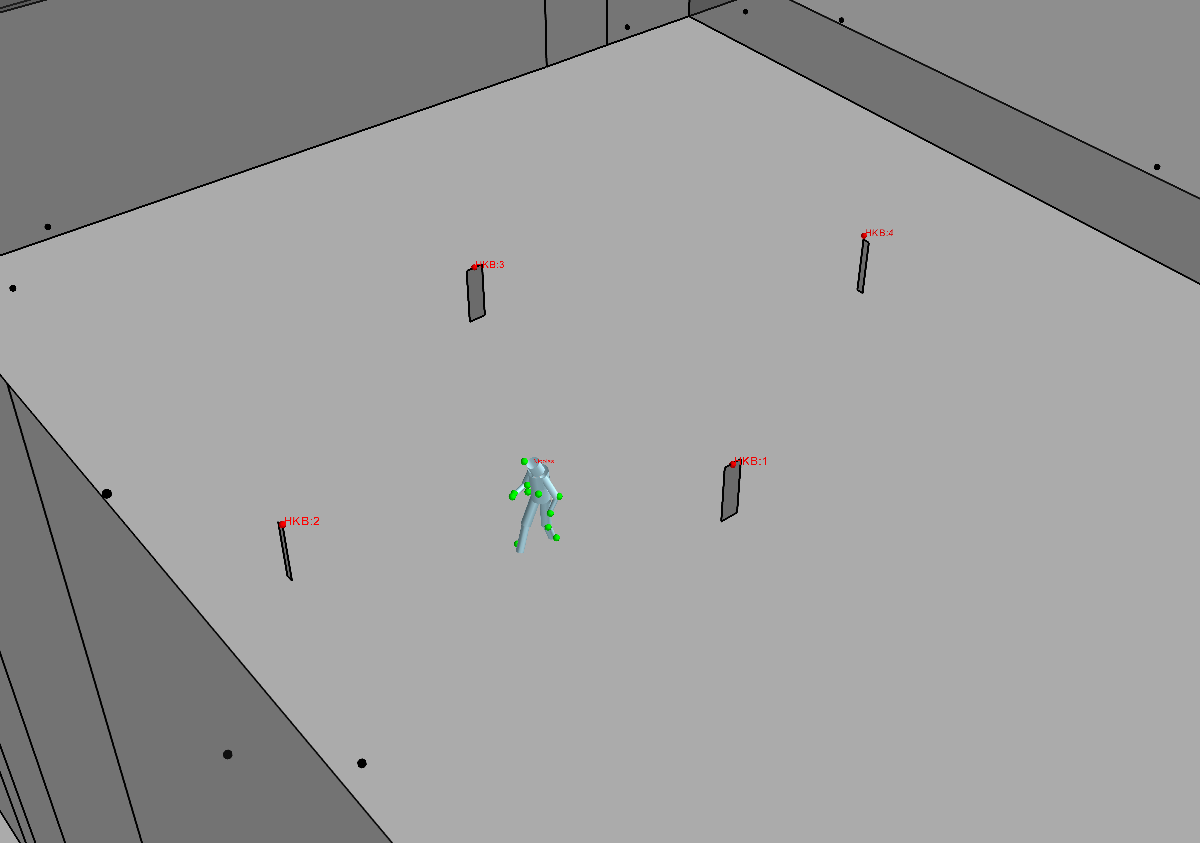
With the help of the Mayavi Library, the CorSer class allows to display in 3D :
The building where measurements have taken place
The positions of Vicon Cameras
The Multi-cylindric representation of the the subjects involved in the selected serie
The position/ antenna pattern of the devices on the body(ies) and in the infrastructure.
By default, the use of the *S._show3* method display the complete scene with body(ies) and associated devices at 4 different timestamp
S._show3()

#the following line is only used to display in the notebook a screenshot of the mayavi window
myu.inotshow('fig1')
/home/uguen/anaconda2/lib/python2.7/site-packages/mayavi/tools/camera.py:288: FutureWarning: elementwise comparison failed; returning scalar instead, but in the future will perform elementwise comparison
  if focalpoint is not None and not focalpoint == 'auto':
Specify time (bodytime parameter)
In order to display scene at specific timestamps, the parameter bodytime can be used
Example: to show the body position at \(t=0s\), \(t=30s\) and \(t=90s\).
S._show3(bodytime=[0.,30.,90.])
#the following line is only used to display in the notebook a screenshot of the mayavi window
myu.inotshow('fig2')
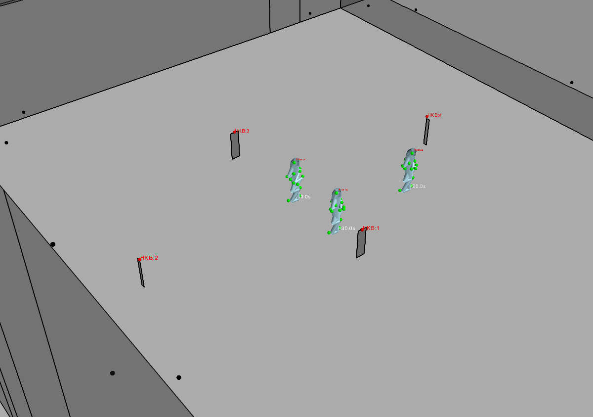
display trajectory (trajectory parameter)
S._show3(trajectory = True,bodytime=[0.,30.,90.])

#the following line is only used to display in the notebook a screenshot of the mayavi window
myu.inotshow('fig3')
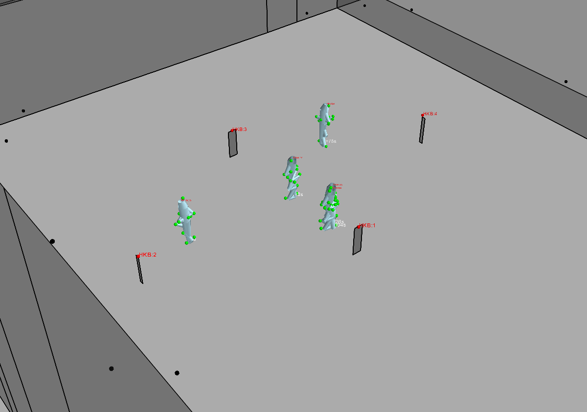
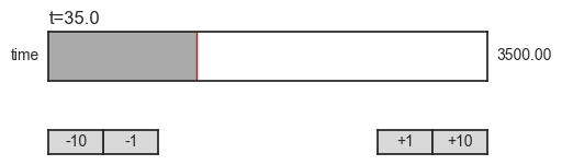
The method *S._show3i()* allows to display the 3D scene with an extra window incluying a slider acting like a jog shuttle, to choose the timestamp to vizualize.
Note : This function is note available in the notebook
S._show3i(t=35) #t=35 is an initialization value

#the following line is only used to display in the notebook a screenshot of the mayavi window
myu.inotshow('fig4')
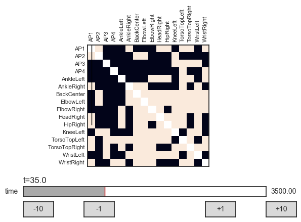
The visibility matrix can be displayed simultaneously to the 3D view.
For that purpose a visibility/occultation matrix is computed the first time the vizualization is called. The following code displays the tisibility matrix and associated 3D scene at the inital time \(t=35s\)
S.imshowvisibility_i(t=35)

#the following line is only used to display in the notebook a screenshot of the mayavi window
myu.inotshow('fig5')
Visibility is computed only once, Please wait

processing shadowing from  Nicolas
Using Pylayers Ray-tracing with CorSer data
import pylayers.simul.simultraj as st
ST = st.Simul(S)
Warning Unable to read graph Gr
Warning Unable to read graph Gw
Layout Graph loaded