Modelisation of the Thermal Noise
from pylayers.signal.bsignal import *
%matplotlib inline
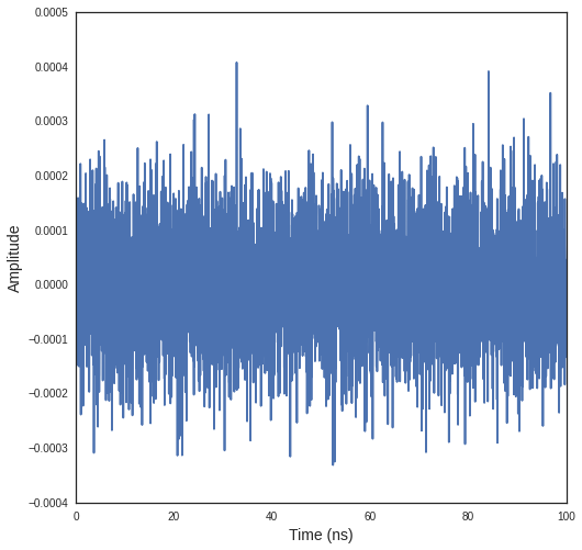
The bsignal module has a dedicated class for handling noise signal. To create a white noise just type :
w = Noise()
The representation of the noise object provides information about
default values. In digital representation of noise the sampling
frequency is important. The noise signal is generated from a time
\(t_i\) to a time \(t_f = t_i+T\). The default power spectral
density is \(-174dBm/Hz\) and can be modified with the argument
PSDdBmpHz.
w
Sampling frequency : 50 GHz
ti  : 0ns
tf  : 100ns
ts  : 0.02ns
N   : 5000
-------------
DSP : -174 dBm/Hz
    : 3.98107170553e-21 Joules
-------------
Noise Figure : 0 dB
Vrms : 9.97631157484e-05 Volts
Variance : 9.47566704228e-09 V^2
Power (dBm) /50 Ohms : -157.010299957 dBm
Power realized /50 Ohms : -157.223602123 dBm
f,a=w.plot(typ='v')
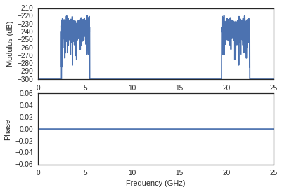
w.psd()
FUsignal : (2500,) (1, 2500)
w2 = w.fgating(fcGHz=4,WGHz=3)
W2=w2.psd()
W2.plotdB(mask=True)
w.plot(typ='v')
(<matplotlib.figure.Figure at 0x7fef5f122190>,
 array([[<matplotlib.axes._subplots.AxesSubplot object at 0x7fef5f1509d0>]], dtype=object))

ip=TUsignal()
ip.EnImpulse(fcGHz=4.4928,WGHz=0.4992,feGHz=100)
#fig = plt.figure(figsize=(10,10))
#for k,snr in enumerate(range(30,-30,-10)):
#    a = fig.add_subplot(3,2,k+1)
#    ipn,n=ip.awgn(snr=snr,typ='snr')
#    ipn.plot(typ='v',fig=fig,ax=a)
#    a.set_title('SNR :'+str(snr)+' dB')
#plt.tight_layout()