!date

samedi 28 avril 2018, 14:09:27 (UTC+0200)

Handling time and frequency domain signals : `Bsignal` Class¶

This section presents some features of the classes implemented in the `pylayers.signal.bsignal.py <http://pylayers.github.io/pylayers/modules/pylayers.signal.bsignal.html>`__ module.

%matplotlib inline

The Bsignal class is a container for a signal with an indexation range which can be either in time domain or frequency domain.

from pylayers.signal.bsignal import *
from matplotlib.pyplot import *

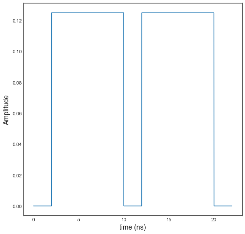
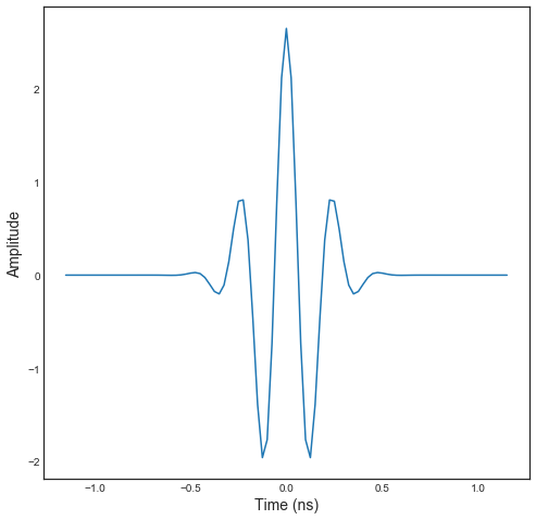
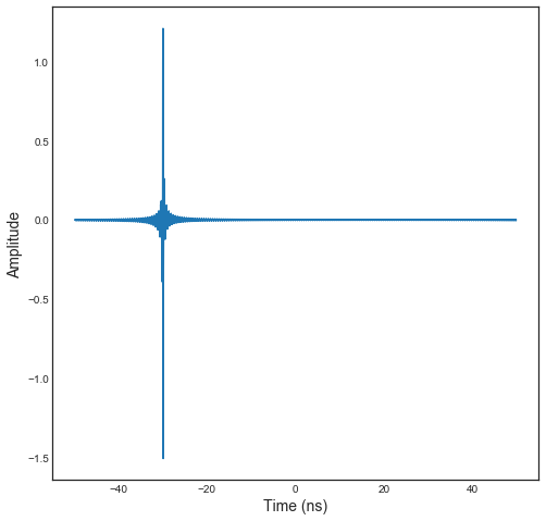
As a first example, let construct an impulse signal normalized in energy. To do so there exist a specialized function : `EnImpulse <http://pylayers.github.io/pylayers/modules/generated/pylayers.signal.bsignal.EnImpulse.demo.html>`__

E=TUsignal()
E.EnImpulse(feGHz=40)

E.plot(typ='v')

(<matplotlib.figure.Figure at 0x7f1cd4a2db70>,
 array([[<matplotlib.axes._subplots.AxesSubplot object at 0x7f1cd4a3d470>]], dtype=object))

E.energy()

array([ 1.00000008])

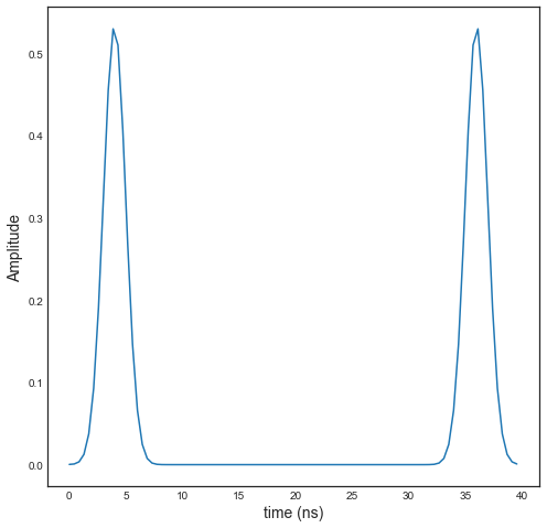
The Fourier transform of this signal exhibits the Hermitian Symmetry.

F = E.fft()
F.plot(typ='m')

(<matplotlib.figure.Figure at 0x7f1cd29faa58>,
 array([[<matplotlib.axes._subplots.AxesSubplot object at 0x7f1cd4a61588>]], dtype=object))

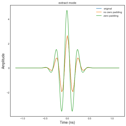
We then extract the non redundant part of the signal with the ft method

G=E.ft()

GH=G.symHz(100,scale='extract')

print(GH.y[0,1])
print(GH.y[0,-1])

(-0.0014441784194-4.88037298122e-05j)
(-0.0014441784194+4.88037298122e-05j)

ip = F.ifft()
ip2= GH.ifft()

f,a=E.plot(typ='v',labels=['original'])
f,a=ip.plot(typ='v',fig=f,ax=a[0][0],labels=['no zero padding'])
f,a=ip2.plot(typ='v',fig=f,ax=a[0][0],labels=['zero padding'])
title('extract mode')

<matplotlib.text.Text at 0x7f1cd28bd080>

ip.energy()

array([ 1.00000008])

ip2.energy()

array([ 3.18478273])

Y=E.esd()

FHsignal in CIR mode¶

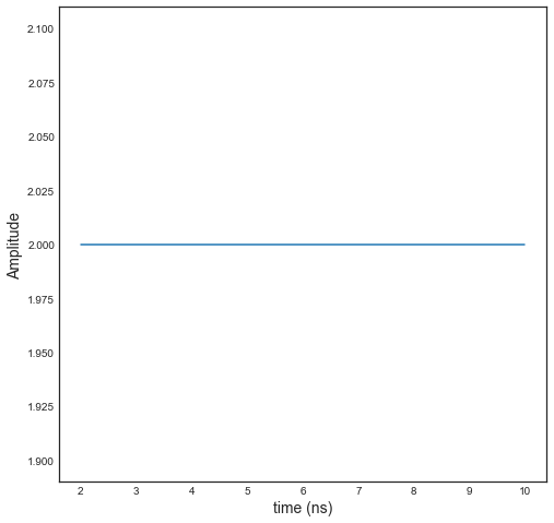
We create a Fusignal which corresponds to the signal

\[X_u(f) = \alpha e^{-2j\pi f \tau}\]

\[f\in [f_{min},f_{max}]\]

fGHz = np.arange(2,10,0.01)
tau = 20
y = 2*np.ones(len(fGHz))*np.exp(-2*1j*np.pi*fGHz*tau)
Hu = FUsignal(fGHz,y)

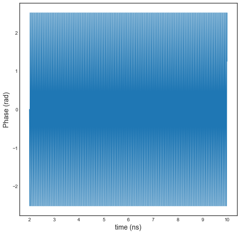
Hu.plot(typ='m')
Hu.plot(typ='r')

(<matplotlib.figure.Figure at 0x7f1cd286e128>,
 array([[<matplotlib.axes._subplots.AxesSubplot object at 0x7f1cd27f02b0>]], dtype=object))

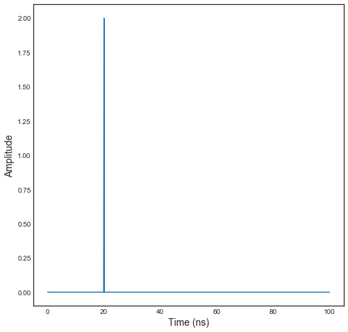
hu = Hu.ifft()

The inverse Fourier transform allows to recover perfectly the amplitude \(\alpha\) and the delay \(\tau\) of the channel

hu.plot(typ='m')

(<matplotlib.figure.Figure at 0x7f1cd2789320>,
 array([[<matplotlib.axes._subplots.AxesSubplot object at 0x7f1cd27e88d0>]], dtype=object))

real=np.imag(hu.y)
u = np.where(hu.y==max(hu.y))[0]
tau = hu.x[u]
alpha = abs(hu.y[u])

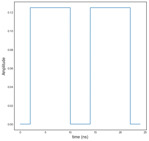
H = Hu.symHz(100,scale='cir')

H.plot(typ='m')

(<matplotlib.figure.Figure at 0x7f1cd2734400>,
 array([[<matplotlib.axes._subplots.AxesSubplot object at 0x7f1cd2797128>]], dtype=object))

h = H.ifft()

h.plot(typ='v')

(<matplotlib.figure.Figure at 0x7f1cd0e6b898>,
 array([[<matplotlib.axes._subplots.AxesSubplot object at 0x7f1cd0f17cc0>]], dtype=object))

real=np.imag(h.y)
u = np.where(h.y==max(h.y))[0]
tau = h.x[u]
alpha = abs(h.y[u])

fft.ifft(H.y)

array([[ -1.50593859e-15 -6.41964563e-20j,
          1.22745263e-04 -1.36427337e-19j,
          8.94216494e-05 -1.03247967e-19j, ...,
          1.05839739e-05 +7.80645228e-20j,
         -1.37135712e-04 -1.94405223e-19j,
          8.17123442e-05 +3.02799103e-19j]])

print(H.y[...,203])
print(H.y[...,-203])
len(H.y)

[-0.10108118-0.07343977j]
[-0.10108118+0.07343977j]

Y=h.fft()

Y.plot(typ='m')

(<matplotlib.figure.Figure at 0x7f1cd0e7c080>,
 array([[<matplotlib.axes._subplots.AxesSubplot object at 0x7f1cd0ec2668>]], dtype=object))

Handling time and frequency domain signals : Bsignal Class¶

FHsignal in CIR mode¶

Handling time and frequency domain signals : `Bsignal` Class¶