!date
dimanche 5 novembre 2017, 20:17:50 (UTC+0100)
Ray Signatures
Signatures are calculated from a cycle to an other cycle of the Layout. They are used for the determination of rays once the transmitter and receiver are known.
The evaluation of a signature from one cycle to another is implemented
in the pylayers.simul.antprop.signature.Signature class.
import time
from pylayers.gis.layout import *
from pylayers.antprop.signature import *
from pylayers.antprop.rays import *
%matplotlib inline
Let load a simple Layout
L = Layout('defstr.lay')
L.build()
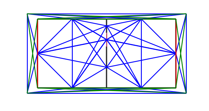
Showing the graph of visibilty
L.showG('sv',figsize=(8,8))
plt.axis('off')
(-2.0, 12.0, -1.0, 6.0)
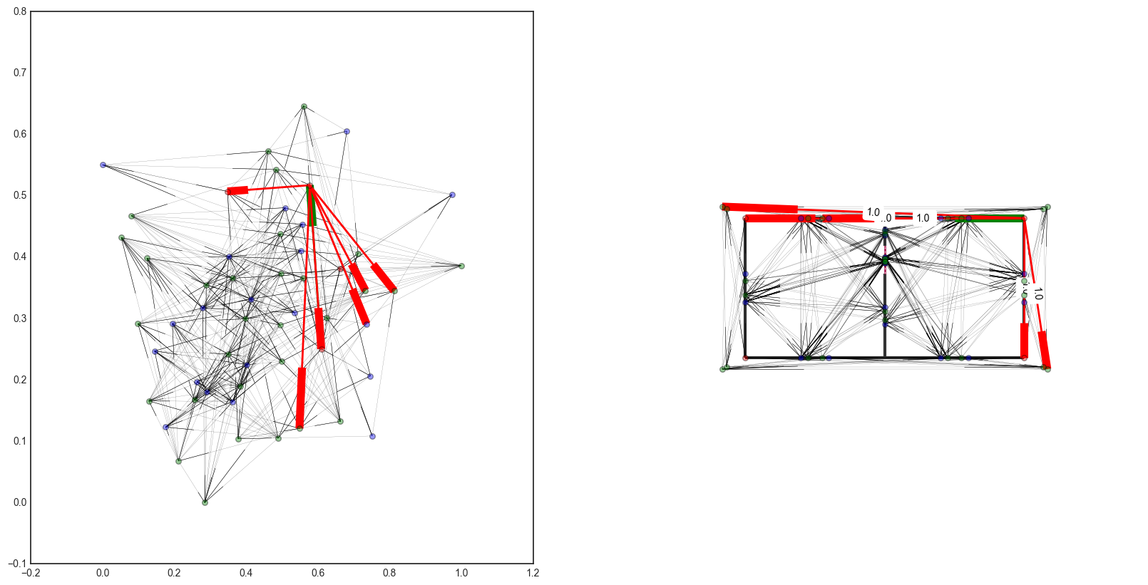
The graph of interactions is shown below :
L._showGi()
(<matplotlib.figure.Figure at 0x7f83e8abe850>,
 <matplotlib.axes._subplots.AxesSubplot at 0x7f83e8c49090>)
<matplotlib.figure.Figure at 0x7f83e8abe850>
The node of Gi are interactions. A transmission is noted Python_
L.Gi.node
{(-6,): {},
 (-4,): {},
 (-3,): {},
 (-1,): {},
 (1, 2): {},
 (1, 2, 5): {},
 (1, 5): {},
 (1, 5, 2): {},
 (2, 2, 5): {},
 (2, 5, 2): {},
 (3, 2): {},
 (3, 2, 5): {},
 (3, 5): {},
 (3, 5, 2): {},
 (4, 2): {},
 (4, 2, 5): {},
 (4, 5): {},
 (4, 5, 2): {},
 (5, 2): {},
 (5, 2, 5): {},
 (5, 5): {},
 (5, 5, 2): {},
 (6, 2): {},
 (6, 2, 4): {},
 (6, 4): {},
 (6, 4, 2): {},
 (7, 1): {},
 (7, 1, 2): {},
 (7, 2): {},
 (7, 2, 1): {},
 (8, 5): {},
 (8, 5, 6): {},
 (8, 6): {},
 (8, 6, 5): {},
 (9, 4): {},
 (9, 4, 5): {},
 (9, 5): {},
 (9, 5, 4): {},
 (10, 2): {},
 (10, 2, 3): {},
 (10, 3): {},
 (10, 3, 2): {},
 (11, 3): {},
 (11, 3, 5): {},
 (11, 5): {},
 (11, 5, 3): {},
 (17, 1, 3): {},
 (17, 3, 1): {},
 (22, 1, 4): {},
 (22, 4, 1): {},
 (28, 3, 6): {},
 (28, 6, 3): {},
 (30, 4, 6): {},
 (30, 6, 4): {}}
All the interactions of a given cycle are stored as meta information in
nodes of Gt
L.Gt.node[1]['inter']
[(15, 1, 0),
 (15, 0, 1),
 (22, 1, 4),
 (22, 4, 1),
 (7, 1),
 (7, 1, 2),
 (7, 2, 1),
 (17, 1, 3),
 (17, 3, 1),
 (-3,),
 (-4,)]
The signature is calculated with as parameters the Layout object and two cycle numbers. In example below it is 0 and 1.
Si = Signatures(L,1,2)
The cold start determination of the signature is done with a run
function. The code is not in its final shape here and there is room for
significant acceleration in incorporating propagation based heuristics.
The mitigation of graph exploration depth is done in setting a
cutoff value which limits the exploration in the interaction graph.
Si.run(cutoff=5,diffraction=False)
Signatures: 100%|??????????????????????????????| 100.0/100 [00:07<00:00, 13.08it/s]
The representation method of a signature gives informations about the different signatures. Signatures are grouped by number of interactions.
L.Gt.pos
{1: array([-0.7826087,  2.5      ]),
 2: array([ 2.5,  2.5]),
 3: array([ 5.        , -0.39130435]),
 4: array([ 5.        ,  5.39130435]),
 5: array([ 7.5,  2.5]),
 6: array([ 10.7826087,   2.5      ])}
ptx = np.array(L.Gt.pos[1])+np.random.rand(2)
prx = np.array(L.Gt.pos[2])+np.random.rand(2)
print ptx
print prx
[-0.09171178  3.49732285]
[ 2.67234051  2.63713575]