The transmission channel
%matplotlib inline
from pylayers.antprop.rays import *
import scipy.fftpack as fft
from pylayers.gis.layout import *
from pylayers.antprop.signature import *
from pylayers.simul.link import *
from pylayers.antprop.channel import *
import pylayers.signal.waveform as wvf
from pylayers.simul.simulem import *
import matplotlib.pyplot as plt
import time
We start by constructing a propagation channel with the dedicated class
DLink. We specify a Layout as well as the two extremities of the
link. Antennas are also specified. The frequency range is determined by
the frequency range of antennas.
L = Layout('defstr.ini')
L.Gs.node[1]['ss_name']=['WOOD','AIR','METAL']
L.build()
tx=array([759,1114,1.0])
rx=array([761,1114,1.5])
fGHz = np.linspace(2,6,401)
Aa = Antenna('Omni',fGHz=fGHz)
Ab = Antenna('Omni',fGHz=fGHz)
Lk = DLink(L=L,a=tx,b=rx,Aa=Aa,Ab=Ab)
building Layout ...
check len(ncycles) == 2 passed
The full evaluation and hdf5 storage of the channel is done with the
eval function. The force option is for forcing a full
reevaluation.
ak,tauk=Lk.eval(force=True)
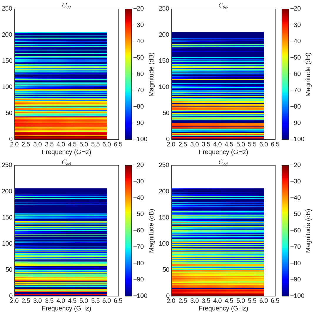
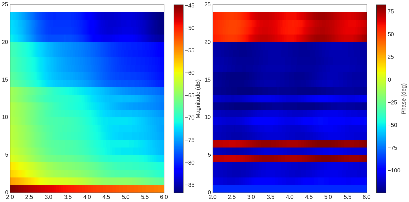
f = plt.figure(figsize=(15,15))
f,a=Lk.C.show(cmap='jet',typ='l20',fig=f,vmin=-100,vmax=-20,fontsize=22)
The transmission channel is stored in H
Lk.H
Tchannel : Ray transfer function (Nray x Nr x Nt x Nf)
-----------------------------------------------------
freq : 2.0 6.0 401
shape  : (206, 1, 1, 401)
tau (min, max) : 6.87184270936 76.4671316464
dist (min,max) : 2.06155281281 22.9401394939
Friis factor -j c/(4 pi f) has been applied
 calibrated : No
 windowed : No
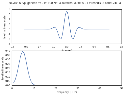
Once the channel has been calculated, we define an Impulse Radio Waveform.
fGHz=np.arange(2,12,.1)
wav = wvf.Waveform(fcGHz=5,bandGHz=3)
wav.show()
is an object which contains all the information about the propagation channel.
f,a=Lk.show()
The Ctilde channel can be sorted with respect to delay
Lk.H
Tchannel : Ray transfer function (Nray x Nr x Nt x Nf)
-----------------------------------------------------
freq : 2.0 6.0 401
shape  : (206, 1, 1, 401)
tau (min, max) : 6.87184270936 76.4671316464
dist (min,max) : 2.06155281281 22.9401394939
Friis factor -j c/(4 pi f) has been applied
 calibrated : No
 windowed : No
len(Lk.fGHz)
402
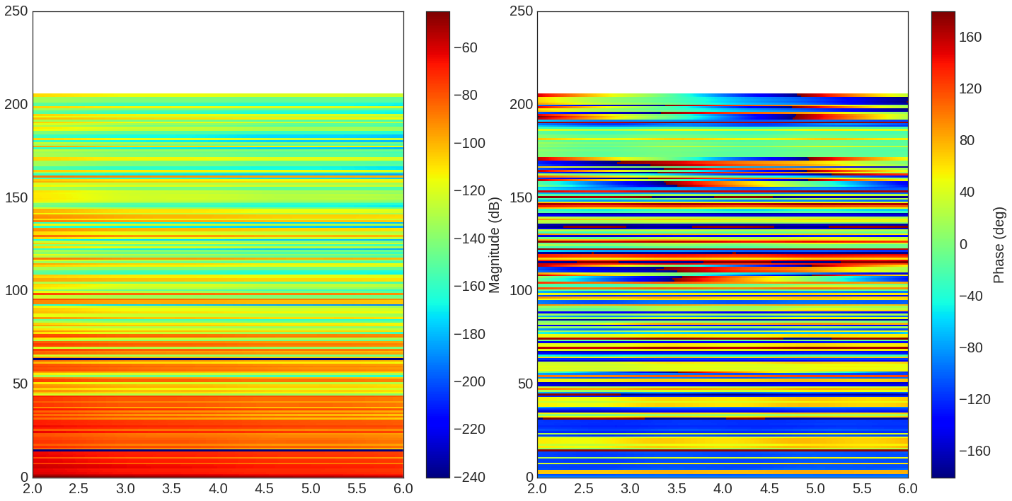
f = plt.figure(figsize=(20,10))
f,a =Lk.H.show(fig=f,cmap='jet')
The Friis factor
The Friis factor is :
This factor is fundamental and has to be applied only once. By default
the link is evaluated with the Friis factor : isFriis=True. This
can be checked at the end of the repr of H.
Lk.H
Tchannel : Ray transfer function (Nray x Nr x Nt x Nf)
-----------------------------------------------------
freq : 2.0 6.0 401
shape  : (206, 1, 1, 401)
tau (min, max) : 6.87184270936 76.4671316464
dist (min,max) : 2.06155281281 22.9401394939
Friis factor -j c/(4 pi f) has been applied
 calibrated : No
 windowed : No
Emean=Lk.H.energy(mode='mean')
Eint=Lk.H.energy(mode='integ')
Ecenter=Lk.H.energy(mode='center')
Efirst=Lk.H.energy(mode='first')
Elast=Lk.H.energy(mode='last')
print Efirst[0],Elast[0]
[[ 3.35253916e-05]] [[ 3.72504352e-06]]
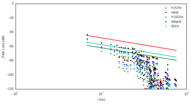
On the figure below we have selected a LOS situation and we compare the energy for each path with the LOS values (the straight line). The 3 straight lines coresponds to the Free space path loss formula for 3 frequencies (f = 2GHz,f=6GHz,f=10GHz). For those 3 frequencies the first path is perfectly on the curve, which is a validation the observed level.
Lk.H.y.shape
(206, 1, 1, 401)
f1 = 2
f2 = 10
f3 = 6
fig = plt.figure(figsize=(10,5))
a = plt.semilogx(Lk.H.taud,10*np.log10(Efirst[:,0,0]),'.r',label='f=2GHz')
a = plt.semilogx(Lk.H.taud,10*np.log10(Emean[:,0,0]),'.b',label='mean')
a = plt.semilogx(Lk.H.taud,10*np.log10(Elast[:,0,0]),'.g',label='f=10GHz')
a = plt.semilogx(Lk.H.taud,10*np.log10(Eint[:,0,0]),'.k',label='integral')
a = plt.semilogx(Lk.H.taud,10*np.log10(Ecenter[:,0,0]),'.c',label='6GHz')
plt.xlabel(r'$\tau$ (ns)')
plt.ylabel('Path Loss (dB)')
LOS1 = -32.4-20*np.log10(Lk.H.taud*0.3)-20*np.log10(f1)
LOS2 = -32.4-20*np.log10(Lk.H.taud*0.3)-20*np.log10(f2)
LOS3 = -32.4-20*np.log10(Lk.H.taud*0.3)-20*np.log10(f3)
plt.semilogx(Lk.H.taud,LOS1,'r')
plt.semilogx(Lk.H.taud,LOS2,'g')
plt.semilogx(Lk.H.taud,LOS3,'c')
plt.semilogx(tauk,20*np.log10(np.sum(np.sum(ak,axis=2),axis=1)),'+')
plt.ylim([-120,0])
plt.legend()
<matplotlib.legend.Legend at 0x7f5539cb78d0>
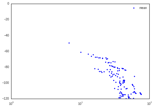
a = plt.semilogx(Lk.H.taud,10*np.log10(Emean[:,0,0]),'.b',label='mean')
plt.semilogx(tauk,20*np.log10(np.sum(np.sum(ak,axis=2),axis=1)),'+')
plt.ylim([-120,0])
plt.legend()
<matplotlib.legend.Legend at 0x7f553b979090>
CIR=TUchannel(tauk,np.zeros(len(tauk)))
CIR.aggcir(ak,tauk)
CIR.stem()
plt.title('Infinite bandwidth CIR')
<matplotlib.text.Text at 0x7f553bb7c650>
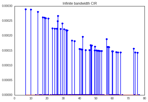
MeanDelay = CIR.tau_moy()
DelaySpread = CIR.tau_rms()
print MeanDelay,DelaySpread
36.619045782 13.4093554011
f = plt.figure(figsize=(20,10))
f=Lk.H.show(cmap='jet',fig=f)

The cut method applies an energy thresholding on the transmission channel.
Lk.H.cut()
f = plt.figure(figsize=(20,10))
f=Lk.H.show(cmap='jet',fig=f)
The tap method
The tap methods takes as parameters : + The system bandwidth \(W\) expressed in MHz + The two extremities velocities \(V_a\) and \(V_b\) + The number of taps to be evaluted \(N_{tap}\) + The number of time samples \(N_m\) + The number of spatial realizations \(N_s\)
This method returns a Multi Dimensional Array \(htap(f,s,m,tap)\)
htap has 4 axes.
axis 0 is frequency,
axis 1 is spatial realization
axis 2 is discrete time
axis 3 is tap index
Va = 10
Vb = 10
fcGHz = 4.5
Nm = 50
Ns = 10
WMHz = 20
Ntap = 10
# htap,b,c,d = Lk.H.tap(WMHz=WMHz,Ns=Ns,Nm=Nm,Va=Va,Vb=Vb,Ntap=Ntap)
#np.shape(htap)
The second parameter is the time integration of htap
axis 0 i frequency
axis 2 is spatial (realization)
axis 2 is tap
# b.shape
# np.shape(c)
# d.shape
The figure below illustrates the joint frequency and spatial fluctuation for the first channel tap. :exit
#img = plt.imshow(abs(b[:,:,0]),interpolation='nearest',extent=(0,1000,fGHz[-1],fGHz[0]))
#plt.axis('tight')
#plt.colorbar()
#plt.xlabel('spatial realizations')
#plt.ylabel('Frequency GHz')
#f = plt.figure(figsize=(10,4))
#h = plt.hist(np.real(b[0,:,0])*1e5,40,normed=True)
#mmax = 0.3*WMHz*1e6/(2*fcGHz*(Va+Vb))
#tmaxms = 1000*mmax/(WMHz*1e6)
#plt.imshow(abs(c[:,:,1]),interpolation='nearest',extent=(0,tmaxms,fGHz[-1],fGHz[0]))
#plt.axis('tight')
#plt.colorbar()
#plt.xlabel('Discrete Time (ms)')
#plt.ylabel('frequency (GHz)')
#plt.plot(abs(c[0,:,0]))
#h = c[:,:,2]
#from pylayers.util.mayautil import *
#m=VolumeSlicer(data=abs(htap[:,0,:,:]))
#m.configure_traits()