Antenna

class pylayers.antprop.antenna.Antenna(typ='Omni', **kwargs)

Bases: pylayers.antprop.antenna.Pattern

name : Antenna name

nf : number of frequency nth : number of theta nph : number of phi

Ft : Normalized Ftheta (ntheta,nphi,nf) Fp : Normalized Fphi (ntheta,nphi,nf) sqG : square root of gain (ntheta,nphi,nf)

theta : theta base 1 x ntheta phi : phi base 1 x phi

C : VSH Coefficients

info : Display information about antenna vsh : calculates Vector Spherical Harmonics show3 : Geomview diagram plot3d : 3D diagram plotting using matplotlib toolkit

Antenna trx file can be stored in various order

natural : HFSS ncp : near filed chamber

It is important when initializing an antenna object to be aware of the typ of trx file

.trx (ASCII Vectorial antenna Pattern)

F Phi Theta Fphi Ftheta

Methods Summary

Fsynth([theta, phi])	Perform Antenna synthesis
Fsynth1(theta, phi)	calculate complex antenna pattern from VSH Coefficients (shape 1)
Fsynth2(theta, phi[, typ])	pattern synthesis from shape 2 vsh coeff
Fsynth2b(theta, phi)	pattern synthesis from shape 2 vsh coefficients
Fsynth2s([dsf])	pattern synthesis from shape 2 vsh coefficients
Fsynth3([theta, phi, typ])	synthesis of a complex antenna pattern from SH coefficients (vsh or ssh in shape 3)
cart2pol(Fx, Fy, Fz, ith)	converts Fx,Fy,Fz to Ftheta, Fphi for theta=ith
checkpole([kf])	display the reconstructed field on pole for integrity verification
coeffshow(**kwargs)	display antenna coefficient
elec_delay(tau)	apply an electrical delay
errel([kf, dsf, typ])	calculates error between antenna pattern and reference pattern
getdelay([delayCandidates])	get electrical delay
info()	gives info about antenna object
initvsh([lmax])	Initialize a void vsh structure
load_atoll([directory])	load antenna from Atoll file
load_trx([directory, nf, ntheta, nphi, ncol])	load a trx file (deprecated)
loadhfss([lfa, Nt, Np])	load antenna from HFSS file
loadmat([directory])	load an antenna stored in a mat file
loadsh2()	load spherical harmonics coefficient in shape 2
loadsh3()	Load antenna’s sh3 file
loadtrx(directory[, param])	load trx file (SATIMO Near Field Chamber raw data)
loadvsh2()	load antenna from .vsh2 file format
loadvsh3()	Load antenna’s vsh3 file
loadvsh3_old()	Load antenna vsh coefficients in shape 3
ls([typ])	list the antenna files in antenna project directory
minsh3([emax])	creates vsh3 with significant coeff until given relative reconstruction error
movie_vsh([mode])	animates vector spherical coeff w.r.t frequency
mse(Fth, Fph[, N])	mean square error between original and reconstructed
pattern([theta, phi, typ])	return multidimensionnal radiation patterns
photo([directory])	show a picture of the antenna
plot3d([k, typ, col])	show 3D pattern in matplotlib
pol2cart(ith)	converts FTheta, FPhi to Fx,Fy,Fz for theta=ith
pol3d([k, R, St, Sp, silent])	Display polarisation diagram in 3D
savesh2()	save coeff in .sh2 antenna file
savesh3()	save antenna in sh3 format
savevsh2([filename])	save coeff in a .vsh2 antenna file
savevsh3([force])	save antenna in vsh3 format
show3([k, po, T, txru, typ, mode, silent])	show3 geomview

Methods Documentation

Fsynth(theta=[], phi=[])

Perform Antenna synthesis

theta : np.array phi : np.array

call Antenna.Fpatt or Antenna.Fsynth3

The antenna pattern synthesis is done either from spherical harmonics coefficients or from an analytical expression of the radiation pattern.

Fsynth1(theta, phi)

calculate complex antenna pattern from VSH Coefficients (shape 1)

theta : ndarray (1xNdir) phi : ndarray (1xNdir) k : int

frequency index

Ft , Fp

Fsynth2(theta, phi, typ='vsh')

pattern synthesis from shape 2 vsh coeff

theta : array 1 x Nt phi : array 1 x Np pattern : boolean

default False

typstring

{vsh | ssh}

Calculate complex antenna pattern from VSH Coefficients (shape 2) for the specified directions (theta,phi) theta and phi arrays needs to have the same size

Fsynth2b(theta, phi)

pattern synthesis from shape 2 vsh coefficients

theta : 1 x Nt phi : 1 x Np

Calculate complex antenna pattern from VSH Coefficients (shape 2) for the specified directions (theta,phi) theta and phi arrays needs to have the same size

Fsynth2s(dsf=1)

pattern synthesis from shape 2 vsh coefficients

phi

Calculate complex antenna pattern from VSH Coefficients (shape 2) for the specified directions (theta,phi) theta and phi arrays needs to have the same size

Fsynth3(theta=[], phi=[], typ='vsh')

synthesis of a complex antenna pattern from SH coefficients (vsh or ssh in shape 3)

Ndir is the number of directions

theta : ndarray (1xNdir if not pattern) (1xNtheta if pattern) phi : ndarray (1xNdir if not pattter) (1xNphi if pattern)

patternboolean

if True theta and phi are reorganized for building the pattern

typ : ‘vsh’ | ‘ssh’ | ‘hfss’

if self.grid:

Fth : ndarray (Ntheta x Nphi) Fph : ndarray (Ntheta x Nphi)

else:

Fth : ndarray (1 x Ndir) Fph : ndarray (1 x Ndir)

pylayers.antprop.channel._vec2scalA

>>> from pylayers.antprop.antenna import *
>>> import numpy as np
>>> import matplotlib.pylab as plt
>>> A = Antenna('defant.vsh3')
>>> F = A.eval(grid=True)

(Source code)

All Br,Cr,Bi,Ci have the same (l,m) index in order to evaluate only once the V,W function

If the data comes from a cst file like the antenna used in WHERE1 D4.1 the pattern is multiplied by $frac{4pi}{120pi}=frac{1}{sqrt{30}$

cart2pol(Fx, Fy, Fz, ith)

converts Fx,Fy,Fz to Ftheta, Fphi for theta=ith

Fx : np.array Fy : np.array Fz : np.array ith : theta index

pol2cart

checkpole(kf=0)

display the reconstructed field on pole for integrity verification

kfint

frequency index default 0

coeffshow(**kwargs)

display antenna coefficient

typstring

‘ssh’ |’vsh’

L : maximum level kf : frequency index vmin : float vmax : float

elec_delay(tau)

apply an electrical delay

taufloat

electrical delay in nanoseconds

This function applies an electrical delay math::exp{+2 j pi f tau) on the phase of diagram math::F_{\theta} and math::F_{phi}

>>> from pylayers.antprop.antenna import *
>>> A = Antenna('S2R2.sh3')
>>> A.eval()
>>> tau = A.getdelay()
>>> A.elec_delay(tau)

(Source code)

errel(kf=-1, dsf=1, typ='s3')

calculates error between antenna pattern and reference pattern

kfinteger

frequency index. If k=-1 integration over all frequency

dsf : down sampling factor typ :

errelThfloat

relative error on \(F_{\theta}\)

errelPhfloat

relative error on \(F_{\phi}\)

errel : float

\[ \begin{align}\begin{aligned}\epsilon_r^{\theta} = \frac{|F_{\theta}(\theta,\phi)-\hat{F}_{\theta}(\theta,\phi)|^2} {|F_{\theta}(\theta,\phi)|^2}\\\epsilon_r^{\phi} = \frac{|F_{\phi}(\theta,\phi)-\hat{F}_{\phi}(\theta,\phi)|^2} {|F_{\theta}(\theta,\phi)|^2}\end{aligned}\end{align} \]

getdelay(delayCandidates=array([-10., -9.999, -9.998, ..., 9.997, 9.998, 9.999]))

get electrical delay

delayCandidatesndarray dalay in (ns)

default np.arange(-10,10,0.001)

electricalDelay : float

AuthorTroels Pedersen (Aalborg University)

B.Uguen

info()

gives info about antenna object

initvsh(lmax=45)

Initialize a void vsh structure

fGHz : array lmax : int

level max

load_atoll(directory='ant')

load antenna from Atoll file

Atoll format provides Antenna gain in the horizontal and vertical plane for different frequencies and different tilt values

directory : string

attol dictionnary is created atoll[keyband][polar][‘hor’] = Ghor.reshape(360,ct,cf) atoll[keyband][polar][‘ver’] = Gver.reshape(360,ct,cf) atoll[keyband][polar][‘tilt’] = np.array(tilt) atoll[keyband][polar][‘freq’] = np.array(tilt)

load_trx(directory='ant', nf=104, ntheta=181, nphi=90, ncol=6)

load a trx file (deprecated)

directorystr

directory where is located the trx file (default : ant)

nffloat

number of frequency points

nthetafloat

number of theta

nphifloat

number of phi

TODO : DEPRECATED (Fix the Ft and Fp format with Nf as last axis)

loadhfss(lfa=[], Nt=72, Np=37)

load antenna from HFSS file

lfa : list of antenna file Nt : int

Number of angle theta

Npint

Number of angle phi

One file per frequency point

th , ph , abs_grlz,th_absdB,th_phase,ph_absdB,ph_phase_ax_ratio

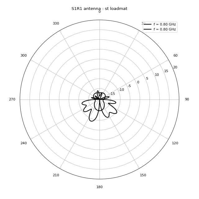
loadmat(directory='ant')

load an antenna stored in a mat file

directorystr , optional

default ‘ant’

>>> import matplotlib.pyplot as plt
>>> from pylayers.antprop.antenna import *
>>> A = Antenna('S1R1.mat',directory='ant/UWBAN/Matfile')
>>> f,a = A.plotG(plan='theta',angdeg=0)
>>> f,a = A.plotG(plan='phi',angdeg=90,fig=f,ax=a)
>>> txt = plt.title('S1R1 antenna : st loadmat')
>>> plt.show()

(Source code)

loadsh2()

load spherical harmonics coefficient in shape 2

loadsh3()

Load antenna’s sh3 file

sh3 file contains a thesholded version of ssh coefficients in shape 3

loadtrx(directory, param={})

load trx file (SATIMO Near Field Chamber raw data)

directory

self._filename: short name of the antenna file

the file is seek in the $BASENAME/ant directory

fmin fmax Nf phmin phmax Nphi thmin thmax Ntheta #EDelay 0 1 2 3 4 5 6 7 8 9 1 10 121 0 6.19 72 0 3.14 37 0

paramdict

mode : string mode 1 : columns are organized [‘f’,’phi’,’th’,’ReFph’,’ImFphi’,’ReFth’,’ImFth’] mode 2 : columns are organized [‘f’,’phi’,’th’,’GdB’,’GdB_ph’,’GdB_th’]

mode2 corresponds to TRXV2

The measured values of Fp Ft and sqG and the associated theta and phi range are stored using the underscore prefix. e.g. self._Ft; self._Fp; self._sqG

for mode 2 : it is require to create a header file “header_<_filename>.txt with the structure # fmin fmax Nf phmin phmax Nphi thmin thmax Ntheta #EDelay and to remove header for trx file.

Warning Mode 2 invert automatocally apply _swap_theta_phi !

loadvsh2()

load antenna from .vsh2 file format

Load antenna’s vsh2 file which only contains the vsh coefficients in shape 2

loadvsh3()

Load antenna’s vsh3 file

vsh3 file contains a thresholded version of vsh coefficients in shape 3

loadvsh3_old()

Load antenna vsh coefficients in shape 3

ls(typ='vsh3')

list the antenna files in antenna project directory

typstring optional

{‘mat’|’trx’|’vsh2’|’sh2’|’vsh3’|’sh3’}

lfile_slist

sorted list of all the .str file of strdir

minsh3(emax=0.05)

creates vsh3 with significant coeff until given relative reconstruction error

emaxfloat

error default 0.05

Create antenna’s vsh3 file which only contains the significant vsh coefficients in shape 3, in order to obtain a reconstruction maximal error = emax

This function requires a reading of .trx file before being executed

movie_vsh(mode='linear')

animates vector spherical coeff w.r.t frequency

modestring

‘linear’ |

mse(Fth, Fph, N=0)

mean square error between original and reconstructed

Fth : np.array Fph : np.array N : int

Calculate the relative mean square error between original pattern A.Ftheta , A.Fphi and the pattern given as argument of the function Fth , Fph

The mse is evaluated on both polarization and normalized over the energy of each original pattern.

The function returns the maximum between those two errors

N is a parameter which allows to suppress value at the pole for the calculation of the error if N=0 all values are kept else N < n < Nt - N

pattern(theta=[], phi=[], typ='s3')

return multidimensionnal radiation patterns

thetaarray

1xNt

phiarray

1xNp

typstring

{s1|s2|s3}

photo(directory='')

show a picture of the antenna

directory : string

plot3d(k=0, typ='Gain', col=True)

show 3D pattern in matplotlib

k : frequency index

typ = ‘Gain’

= ‘Ftheta’ = ‘Fphi’

if col -> color coded plot3D else -> simple plot3D

pol2cart(ith)

converts FTheta, FPhi to Fx,Fy,Fz for theta=ith

ith : theta index

Fx Fy Fz

cart2pol

pol3d(k=0, R=50, St=4, Sp=4, silent=False)

Display polarisation diagram in 3D

kint

frequency index

Rfloat

radius of the sphere

Stint

downsampling factor along theta

Spint

downsampling factor along phi

silentBoolean

(if True the file is created and not displayed’)

The file created is named : Polar{ifreq}.list it is placed in the /geom directory of the project

savesh2()

save coeff in .sh2 antenna file

savesh3()

save antenna in sh3 format

create a .sh3 antenna file

savevsh2(filename='')

save coeff in a .vsh2 antenna file

filename : string

savevsh3(force=False)

save antenna in vsh3 format

Create a .vsh3 antenna file

show3(k=0, po=[], T=[], txru=0, typ='G', mode='linear', silent=False)

show3 geomview

k : frequency index po : poition of the antenna T : GCS of the antenna typ : string

‘G’ | ‘Ft’ | ‘Fp’

modestring

‘linear’| ‘not implemented’

silentboolean

True | False

>>> from pylayers.antprop.antenna import *
>>> import numpy as np
>>> import matplotlib.pylab as plt
>>> A = Antenna('defant.sh3')
>>> #A.show3()