cost231

pylayers.antprop.loss.cost231(pBS, pMS, hroof, phir, wr, fMHz, wb=20, dB=True, city='medium')

Walfish Ikegami model (COST 231)

pBS : np.array (3xNlink) pMS : np.array (3xNlink) hroof : np.array (1xNlink) phir : np.array (1xNlink)

degrees

wr : np.array (1xNlink) fMHz : np.array (1xNf) wb : float

average building separation

dB : boolean

PathLoss (Nlink,Nf)

http://morse.colorado.edu/~tlen5510/text/classwebch3.html

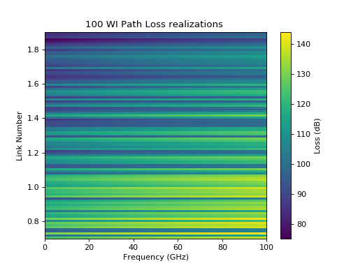
>>> from pylayers.antprop.loss import *
>>> import matplotlib.pyplot as plt
>>> import numpy as np
>>> # Number of links and BS and MS heights
>>> Nlink = 100
>>> hBS = 300
>>> hMS = 1.5
>>> # hroof and phir are drawn uniformily at random 
>>> hroof = 40*np.random.rand(Nlink)
>>> wr = 10*np.ones(Nlink)
>>> phir = 90*np.random.rand(Nlink)
>>> pMS = np.vstack((np.linspace(10,2500,Nlink),np.zeros(Nlink),hMS*np.ones(Nlink)))
>>> pBS = np.vstack((np.zeros(Nlink),np.zeros(Nlink),hBS*np.ones(Nlink)))
>>> # frequency range 
>>> fMHz = np.linspace(700,1900,120)
>>> pl = cost231(pBS,pMS,hroof,phir,wr,fMHz)
>>> im = plt.imshow(pl,extent=(0,100,0.7,1.9))
>>> cb = plt.colorbar()
>>> cb.set_label('Loss (dB)')
>>> plt.axis('tight')
>>> plt.xlabel('Frequency (GHz)')
>>> plt.ylabel('Link Number')
>>> plt.title('100 WI Path Loss realizations ')
>>> plt.show()

(Source code)