The class Cone
>>> from pylayers.util.cone import *
>>> from pylayers.util.geomutil import *
>>> from pylayers.util.plotutil import *
>>> %matplotlib inline
The `Cone <http://pylayers.github.io/pylayers/modules/pylayers.util.cone.html>`__ class implements several methods for handling planar cones.
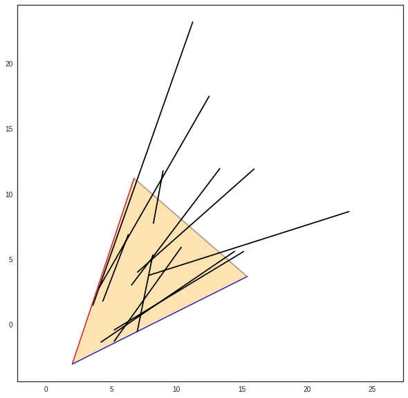
A planar cone is defined as being composed of : + an apex + two vectors and not necessarily normalized.
Let create a cone.
>>> va = np.array([2,1])
>>> vb = np.array([1,3])
>>> C = Cone(va,vb,apex=np.array([2,-3]))
From those parameters the Cone __init__ constructs 2 unitary vectors and such that :
This can be interpreted as applying an anticlockwise rotation from to .
>>> print "Unitary vector u",C.u
>>> print "Unitary vector v",C.v
>>> print "dot(u,v)",C.dot
>>> print "cross(u,v)",C.cross
Unitary vector u [ 0.89442719  0.4472136 ]
Unitary vector v [ 0.31622777  0.9486833 ]
dot(u,v) 0.707106781187
cross(u,v) 0.707106781187
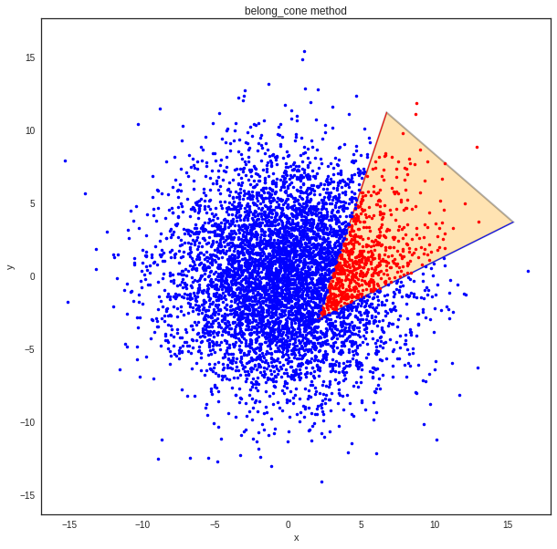
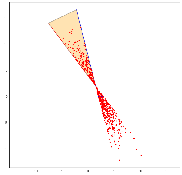
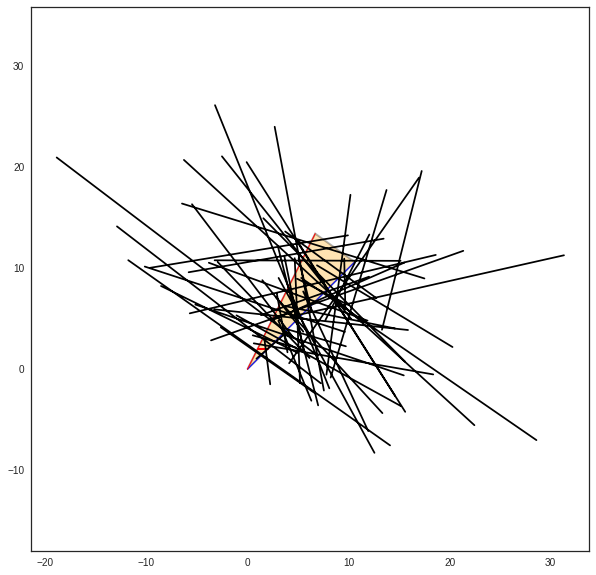
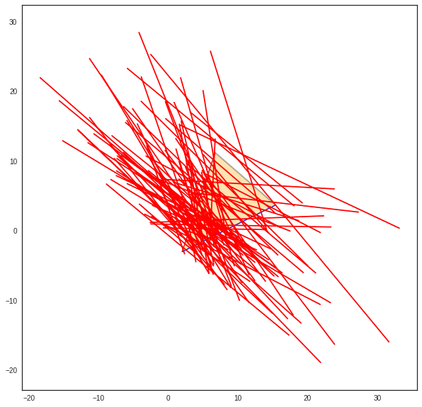
Is a point belonging to a cone ? : belong_point()
>>> p = 4*np.random.randn(2,6000)
>>> b = C.belong_point(p)
>>> nb = np.array(map(lambda x: not x,b))
>>> pr = p[:,b]
>>> pb = p[:,nb]
>>> fig,ax = C.show()
>>> ax.plot(pr[0,:],pr[1,:],'.r')
>>> ax.plot(pb[0,:],pb[1,:],'.b')
>>> plt.axis('equal')
>>> plt.title('belong_cone method')
>>> plt.xlabel('x')
>>> plt.ylabel('y')
>>> #plt.axis('off')
<matplotlib.text.Text at 0x7f9c2a396790>
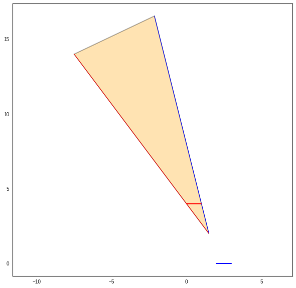
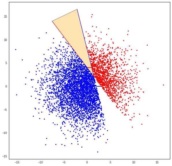
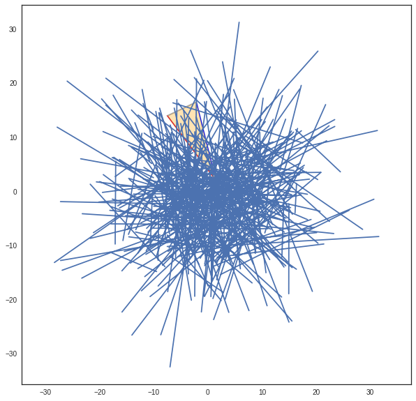
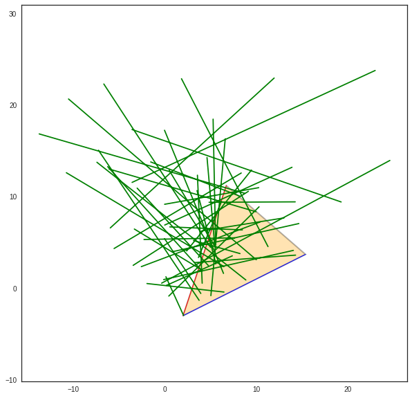
Creating a Cone from 2 segments from2segs()
>>> seg0 = np.array([[2,3],[0,0]])
>>> seg1 = np.array([[0,1],[4,4]])
>>> Cs=Cone()
>>> Cs.from2segs(seg0,seg1)
>>> Cs.apex
array([ 1.5, 2. ])
>>> Cs.seg1-seg1
array([[0, 0],
       [0, 0]])
>>> Cs.show()
(<matplotlib.figure.Figure at 0x7f9c29ece150>,
 <matplotlib.axes._subplots.AxesSubplot at 0x7f9c2a2ad350>)
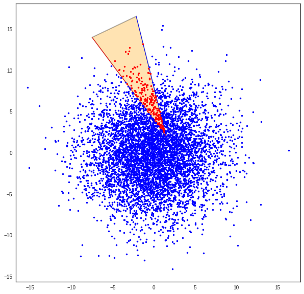
>>> b=Cs.belong_point(p)
>>> pta = 10*sp.randn(2,1000)
>>> phe = 10*sp.randn(2,1000)
>>> nb = np.array(map(lambda x: not x,b))
>>> pr = p[:,b]
>>> pb = p[:,nb]
>>> fig,ax = Cs.show()
>>> #displot(pta[:,bs],phe[:,bs],color='k')
... ax.plot(pr[0,:],pr[1,:],'.r')
>>> ax.plot(pb[0,:],pb[1,:],'.b')
>>> plt.axis('equal')
>>> #plt.axis('off')
(-16.910598251516173,
 17.99623744471733,
 -15.60365452654651,
 18.083365694024096)
>>> Cs.seg1
array([[0, 1],
       [4, 4]])
>>> bi=Cs.belong_point2(p)
>>> %timeit b=Cs.belong_point(p)
The slowest run took 5.18 times longer than the fastest. This could mean that an intermediate result is being cached.
10000 loops, best of 3: 107 µs per loop
>>> #nb = np.array(map(lambda x: not x,bo))
... pr = p[:,bi]
>>> #pb = p[:,bo2]
... fig,ax = Cs.show()
>>> ax.plot(pr[0,:],pr[1,:],'.r')
>>> #ax.plot(pb[0,:],pb[1,:],'.b')
... plt.axis('equal')
>>> #plt.axis('off')
(-8.383229151638302,
 11.047812184404364,
 -13.578383241089245,
 17.986924204240417)
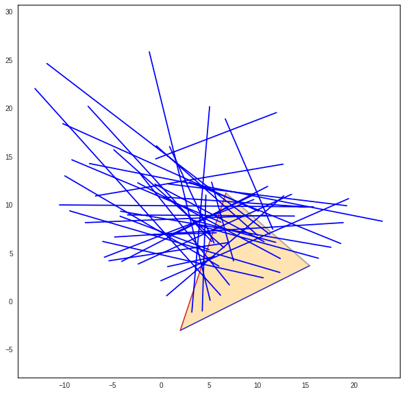
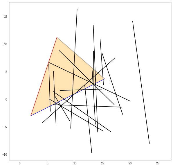
The adressed problem consists in determining whether a segment lies in the cone or not. The condition is satisfied if not all segments termination are outside the cone on the same side of the cone. This is implemented in the method Cone.outside
>>> b1,b2=Cs.outside_point(p)
>>> pr = p[:,b1]
>>> pb = p[:,b2]
>>> fig,ax = Cs.show()
>>> ax.plot(pr[0,:],pr[1,:],'.r')
>>> ax.plot(pb[0,:],pb[1,:],'.b')
>>> plt.axis('equal')
>>> #plt.axis('off')
(-16.910598251516173,
 17.99623744471733,
 -15.60365452654651,
 18.083365694024096)
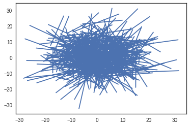
Un cone est un objet qui va servir construire les objets Beams. Un Beam est un Cone qui englobe les segments d’une Signature. Une signature et un point donne un Beam. A un Beam est associ un Cone dont l’apex est une ancre virtuelle.
>>> pta = 10*sp.randn(2,400)
>>> phe = 10*sp.randn(2,400)
>>> displot(pta,phe)
(<matplotlib.figure.Figure at 0x7f9c2a134290>,
 <matplotlib.axes._subplots.AxesSubplot at 0x7f9c2a1f0210>)
>>> Cs.seg0
array([[2, 3],
       [0, 0]])
>>> typ, proba = Cs.belong_seg(pta,phe)
>>> fig,ax = Cs.show()
>>> bs1 = np.where(typ==1)[0]
>>> bs2 = np.where(typ==2)[0]
>>> bs3 = np.where(typ==3)[0]
>>> bs4 = np.where(typ==4)[0]
>>> bs5 = np.where(typ==5)[0]
>>> bs6 = np.where(typ==6)[0]
>>> displot(pta[:,bs1],phe[:,bs1],color='g')
>>> displot(pta[:,bs2],phe[:,bs2],color='b')
>>> displot(pta[:,bs3],phe[:,bs3],color='b')
>>> displot(pta[:,bs4],phe[:,bs4],color='r')
>>> displot(pta[:,bs5],phe[:,bs5],color='r')
>>> #displot(pta[:,bs6],phe[:,bs6],color='m')
... #displot(pta[:,bs],phe[:,bs],color='blue')
(<matplotlib.figure.Figure at 0x7f9c2a10c550>,
 <matplotlib.axes._subplots.AxesSubplot at 0x7f9c2a04cbd0>)
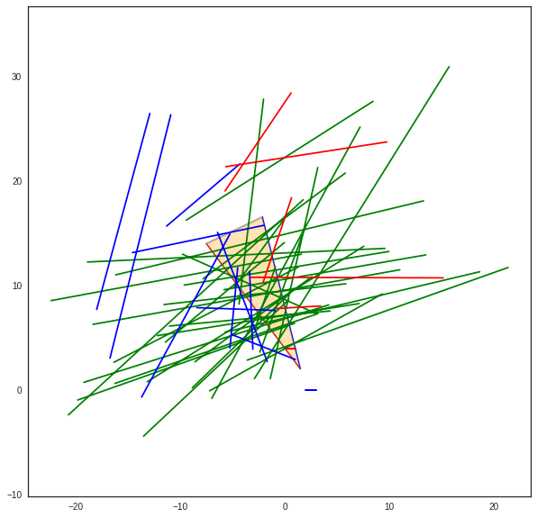
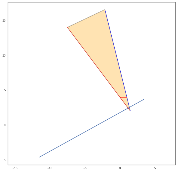
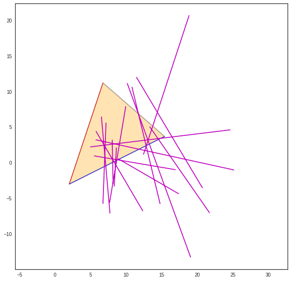
There is different way to create a Cone either from 2 segments from2segs or from one point and one segment fromptseg. This second method is used when the field is going from a diffraction point to a segment.
Conditional Graph
is a conditional graph meaning that the edge indicates which is the list of authorized next edge for the output. A ray being a sequence of nodes of . The cone angular sector represents the whole set and each intercepting segment, is a part or this whole set. This can be interpreted as a probability. This means that the research of rays could be done stochastically in a very efficient manner. This is not fully implemented yet.
>>> Cb = Cone()
>>> Cb.u
array([ 1., 0.])
>>> seg = np.array([[1,2],[2,2]])
>>> pt = np.array([0,0])
>>> Cb.fromptseg(pt,seg)
>>> typ,proba = Cb.belong_seg(pta,phe)
>>> bs = np.where(typ>0)[0]
>>> Cb.seg1
array([[1, 2],
       [2, 2]])
>>> Cb.show()
>>> displot(pta[:,bs],phe[:,bs],color='k')
(<matplotlib.figure.Figure at 0x7f9c2a116b10>,
 <matplotlib.axes._subplots.AxesSubplot at 0x7f9c29fd2150>)
Benchmark normalizing a vector
>>> a = np.array([5,6])
>>> %timeit a/np.sqrt(np.dot(a,a))
The slowest run took 16.64 times longer than the fastest. This could mean that an intermediate result is being cached.
100000 loops, best of 3: 5.17 µs per loop
>>> %timeit a/sp.linalg.norm(a)
The slowest run took 5.60 times longer than the fastest. This could mean that an intermediate result is being cached.
100000 loops, best of 3: 10.9 µs per loop
>>> %timeit a/np.sqrt(np.sum(a*a,axis=0))
The slowest run took 4.79 times longer than the fastest. This could mean that an intermediate result is being cached.
100000 loops, best of 3: 10.1 µs per loop
Debug
This a case which where segments seg0 and seg1 are orthogonal
>>> seg0 = array([[-25.768, -25.822],
...        [  4.28 ,   9.925]])
NameErrorTraceback (most recent call last)

<ipython-input-39-1063b62b8faf> in <module>()
----> 1 seg0 = array([[-25.768, -25.822],
      2        [  4.28 ,   9.925]])


NameError: name 'array' is not defined
>>> seg1 = array([[-26.848, -26.805],
...        [  5.415,   4.515]])
NameErrorTraceback (most recent call last)

<ipython-input-40-95e9502a4505> in <module>()
----> 1 seg1 = array([[-26.848, -26.805],
      2        [  5.415,   4.515]])


NameError: name 'array' is not defined
>>> cn = Cone()
>>> cn.from2segs(seg0,seg1)
>>> pta =array([[-27.836, -27.833, -27.833, -27.817, -26.848, -27.774, -26.952,
...         -28.062],
...        [ 10.926,  10.686,  10.686,   8.956,   5.415,   4.506,  10.934,    8.954]])
NameErrorTraceback (most recent call last)

<ipython-input-43-b197e999ada8> in <module>()
----> 1 pta =array([[-27.836, -27.833, -27.833, -27.817, -26.848, -27.774, -26.952,
      2         -28.062],
      3        [ 10.926,  10.686,  10.686,   8.956,   5.415,   4.506,  10.934,    8.954]])


NameError: name 'array' is not defined
>>> phe = array([[-27.835, -27.835, -28.078, -27.774, -26.882, -26.805, -27.836,
...         -28.078],
...        [ 10.891,  10.891,  10.683,   4.506,   8.965,   4.515,  10.926,
...          10.683]])
NameErrorTraceback (most recent call last)

<ipython-input-44-b4e3a2a92cdb> in <module>()
----> 1 phe = array([[-27.835, -27.835, -28.078, -27.774, -26.882, -26.805, -27.836,
      2         -28.078],
      3        [ 10.891,  10.891,  10.683,   4.506,   8.965,   4.515,  10.926,
      4          10.683]])


NameError: name 'array' is not defined
>>> typ,proba = cn.belong_seg(pta,phe)
>>> bn = np.where(typ==0)[0]
>>> proba
array([ 0.        ,  0.40743308,  1.        ,  0.        ,  0.        ,
        0.        ,  0.        ,  1.        ,  0.        ,  0.        ,
        0.        ,  0.        ,  0.        ,  0.        ,  0.        ,
        0.        ,  0.        ,  0.        ,  0.        ,  0.        ,
        0.        ,  0.        ,  0.        ,  0.        ,  0.        ,
        0.        ,  0.        ,  0.        ,  0.        ,  0.        ,
        0.        ,  0.        ,  0.        ,  0.        ,  0.        ,
        0.        ,  0.        ,  0.        ,  0.        ,  0.        ,
        0.        ,  0.        ,  0.        ,  0.        ,  0.        ,
        0.        ,  0.        ,  0.        ,  0.        ,  0.        ,
        0.        ,  1.        ,  0.        ,  0.        ,  0.27882553,
        0.        ,  0.        ,  0.        ,  0.        ,  0.        ,
        0.        ,  0.        ,  0.        ,  0.        ,  0.        ,
        0.        ,  0.70258493,  0.        ,  0.        ,  0.        ,
        0.        ,  0.        ,  0.        ,  0.        ,  0.        ,
        0.        ,  0.        ,  0.        ,  0.        ,  0.        ,
        0.        ,  0.        ,  0.        ,  0.        ,  0.        ,
        0.        ,  0.        ,  0.        ,  0.        ,  0.        ,
        0.        ,  0.        ,  0.        ,  0.        ,  0.        ,
        0.        ,  1.        ,  1.        ,  0.        ,  0.        ,
        0.        ,  0.        ,  0.        ,  0.        ,  0.        ,
        0.        ,  0.        ,  0.        ,  1.        ,  0.        ,
        0.        ,  0.        ,  0.        ,  0.        ,  0.        ,
        0.        ,  0.        ,  0.        ,  1.        ,  0.        ,
        0.        ,  0.        ,  0.        ,  0.        ,  0.        ,
        1.        ,  1.        ,  1.        ,  0.        ,  0.        ,
        0.        ,  0.        ,  0.        ,  0.        ,  0.        ,
        0.        ,  0.        ,  0.        ,  0.        ,  0.        ,
        0.        ,  0.        ,  0.        ,  0.4118138 ,  0.        ,
        0.        ,  0.        ,  0.        ,  0.        ,  0.        ,
        0.        ,  0.        ,  0.        ,  0.        ,  0.        ,
        0.        ,  0.        ,  0.        ,  0.        ,  0.        ,
        1.        ,  0.        ,  0.        ,  0.        ,  0.        ,
        0.        ,  0.        ,  0.        ,  0.        ,  0.        ,
        0.        ,  0.        ,  0.        ,  0.        ,  0.        ,
        0.        ,  0.        ,  0.        ,  0.        ,  0.        ,
        0.60091961,  1.        ,  0.        ,  0.        ,  0.        ,
        0.        ,  0.        ,  0.        ,  0.        ,  0.        ,
        0.        ,  1.        ,  0.72712004,  0.        ,  1.        ,
        0.        ,  0.        ,  0.        ,  0.        ,  0.        ,
        0.        ,  0.        ,  0.        ,  1.        ,  0.        ,
        0.        ,  0.        ,  0.        ,  0.        ,  0.        ,
        1.        ,  0.        ,  0.        ,  0.        ,  0.        ,
        0.        ,  0.        ,  0.58889221,  0.        ,  0.        ,
        0.        ,  0.        ,  0.        ,  0.        ,  0.        ,
        0.        ,  0.37204381,  0.        ,  0.        ,  0.        ,
        0.        ,  0.        ,  0.        ,  0.        ,  0.        ,
        1.        ,  0.        ,  0.        ,  0.        ,  0.        ,
        1.        ,  0.        ,  0.        ,  0.        ,  0.        ,
        0.        ,  0.        ,  0.        ,  0.        ,  0.43184077,
        0.        ,  0.        ,  0.        ,  1.        ,  0.        ,
        0.        ,  1.        ,  0.        ,  0.        ,  0.        ,
        0.19774672,  0.        ,  0.        ,  0.        ,  0.        ,
        0.        ,  0.        ,  0.        ,  0.2268908 ,  0.        ,
        0.61074076,  0.        ,  0.        ,  0.        ,  0.        ,
        0.        ,  0.        ,  0.        ,  0.        ,  1.        ,
        0.        ,  0.        ,  0.        ,  0.        ,  0.        ,
        0.        ,  0.        ,  0.        ,  0.        ,  0.        ,
        0.        ,  0.        ,  0.        ,  0.        ,  1.        ,
        0.        ,  0.        ,  0.        ,  0.        ,  0.        ,
        0.        ,  0.        ,  0.        ,  0.        ,  0.        ,
        0.        ,  1.        ,  0.        ,  0.24722323,  0.        ,
        0.        ,  0.        ,  0.        ,  0.        ,  0.        ,
        0.        ,  1.        ,  0.        ,  0.        ,  0.        ,
        0.        ,  0.        ,  0.89380205,  0.        ,  1.        ,
        0.        ,  0.        ,  0.        ,  1.        ,  0.        ,
        0.        ,  0.        ,  0.        ,  0.        ,  0.        ,
        0.        ,  1.        ,  0.99196169,  0.        ,  0.        ,
        1.        ,  0.        ,  0.        ,  0.        ,  0.        ,
        0.        ,  0.        ,  0.        ,  1.        ,  0.        ,
        0.        ,  0.        ,  0.        ,  0.        ,  0.        ,
        0.        ,  1.        ,  0.        ,  0.        ,  0.        ,
        0.        ,  1.        ,  0.        ,  0.37718956,  0.        ,
        0.        ,  0.        ,  0.        ,  0.        ,  0.        ,
        0.        ,  0.        ,  0.        ,  0.        ,  0.        ,
        0.        ,  0.        ,  0.        ,  0.        ,  0.        ,
        0.        ,  0.        ,  0.        ,  1.        ,  0.        ,
        0.        ,  0.        ,  0.        ,  0.        ,  0.61405648,
        0.        ,  0.        ,  0.        ,  0.        ,  0.        ,
        0.        ,  0.        ,  0.        ,  0.        ,  0.        ])
>>> cn.show()
>>> displot(pta[:,bn],phe[:,bn])
(<matplotlib.figure.Figure at 0x7f9c2a137550>,
 <matplotlib.axes._subplots.AxesSubplot at 0x7f9c2a1561d0>)
>>> pta1=pta[:,5].reshape(2,1)
>>> phe1=phe[:,5].reshape(2,1)
>>> cn.show()
>>> displot(pta1,phe1)
(<matplotlib.figure.Figure at 0x7f9c2833b190>,
 <matplotlib.axes._subplots.AxesSubplot at 0x7f9c283be890>)
>>> b = cn.belong_seg(pta1,phe1)
geomutil.mirror
>>> p = np.random.randn(2,10000)
>>> pa  = np.array([-1,1]).reshape(2,1)
>>> pb  = np.array([-1,3]).reshape(2,1)
>>> M = geu.mirror(p,pa,pb)
>>> M
array([[-1.80056506, -0.45566959, -2.57142226, ..., -2.0853822 ,
        -2.38869618, -2.88978071],
       [-1.3130668 , -0.8099664 , -0.45534988, ..., -0.01105269,
        -0.64514099, -0.53957856]])
>>> figsize(20,20)
>>> displot(pa,pb)
>>> plot(p[0,:],p[1,:],'or',alpha=0.2)
>>> plot(M[0,:],M[1,:],'ob',alpha=0.2)
NameErrorTraceback (most recent call last)

<ipython-input-53-0829430ac458> in <module>()
----> 1 figsize(20,20)
      2 displot(pa,pb)
      3 plot(p[0,:],p[1,:],'or',alpha=0.2)
      4 plot(M[0,:],M[1,:],'ob',alpha=0.2)


NameError: name 'figsize' is not defined
>>> pa=np.array([0,0]).reshape(2,1)
>>> pb=np.array([1,0]).reshape(2,1)
>>> pc=np.array([1,0]).reshape(2,1)
>>> geu.isaligned(pa,pb,pc)
array([ True], dtype=bool)
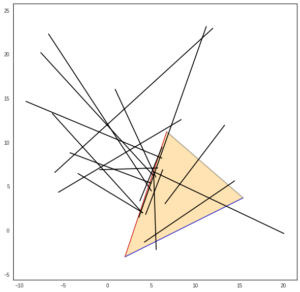
Geometric probability
The idea is to add an information of the fraction of the angular sector which is subtended by the intercepted segment.
>>> a = np.array([2,1])
>>> b = np.array([1,3])
>>> C = Cone(a,b,apex=np.array([2,-3]))
>>> import scipy as sp
>>> pta = np.array([2,-1]).reshape(2,1)
>>> phe = np.array([5.99,-1]).reshape(2,1)
>>> pta = 10*sp.randn(2,1000)
>>> phe = 10*sp.randn(2,1000)
>>> typ,proba = C.belong_seg(pta,phe)
>>> u0 = np.where(typ==0)[0]
>>> u1 = np.where(typ==1)[0]
>>> u2 = np.where(typ==2)[0]
>>> u3 = np.where(typ==3)[0]
>>> u4 = np.where(typ==4)[0]
>>> u5 = np.where(typ==5)[0]
>>> u6 = np.where(typ==6)[0]
>>> us = np.where( ((proba<0.1) & (proba>0)) )  [0]
>>> C.show()
>>> #col=['r','g','b','m']
... try:
...     displot(pta[:,us],phe[:,us],color='k')
>>> except:
...     pass
>>> C.show()
>>> #col=['r','g','b','m']
... try:
...     displot(pta[:,u1],phe[:,u1],color='r')
>>> except:
...     pass
>>> print proba[u1]
[ 1.  1.  1.  1.  1.  1.  1.  1.  1.  1.  1.  1.  1.  1.  1.  1.  1.  1.
  1.  1.  1.  1.  1.  1.  1.  1.  1.  1.  1.  1.  1.  1.  1.  1.  1.  1.
  1.  1.  1.  1.  1.  1.  1.  1.  1.  1.  1.  1.  1.  1.  1.  1.  1.  1.
  1.  1.  1.  1.  1.  1.  1.  1.  1.  1.  1.  1.  1.  1.  1.  1.  1.  1.
  1.  1.  1.  1.  1.  1.  1.  1.  1.  1.  1.  1.]
>>> C.show()
>>>
>>> try:
...     displot(pta[:,u2],phe[:,u2],color='g')
>>> except:
...     pass
>>> print(proba[u2])
[ 0.43736156  0.06870599  0.46854134  0.26991912  0.96209565  0.79693702
  0.36749495  0.18412835  0.97480557  0.46713302  0.61805484  0.13551922
  0.3975633   0.47553598  0.92331495  0.5629051   0.75990021  0.44981204
  0.15474131  0.05718427  0.3077045   0.07986304  0.0765847   0.72161955
  0.12242633  0.53618313  0.91036233  0.93245053  0.61131975  0.15680479
  0.0842943   0.37081325  0.00483835  0.33803883  0.20684903  0.79545636
  0.7712438   0.15038099  0.73535369  0.18306744  0.27086345  0.36148261
  0.58175241]
>>> C.show()
>>> try:
...     displot(pta[:,u3],phe[:,u3],color='b')
>>> except:
...     pass
>>> print(proba[u3])
[ 0.53321774  0.2850624   0.79714699  0.66820213  0.46329356  0.02231597
  0.6381687   0.94873691  0.06028365  0.42577666  0.40170715  0.87097009
  0.28018797  0.60192762  0.77218623  0.46068757  0.24231895  0.12012527
  0.2958268   0.02564258  0.20903551  0.5848245   0.54536372  0.6756437
  0.14882913  0.95825158  0.55487465  0.91997086  0.58973664  0.97724919
  0.42385107  0.04634142  0.63801452  0.22673842  0.32913638  0.04037261
  0.95984203  0.84635994  0.31051312  0.64204187  0.22578098  0.74498622]
>>> C.show()
>>> try:
...     displot(pta[:,u4],phe[:,u4],color='m')
>>> except:
...     pass
>>> print(proba[u4])
[ 0.28172671  0.25177525  0.75563027  0.57569771  0.98287884  0.19041544
  0.32268279  0.80352579  0.37777776  0.51817355  0.39252555  0.25674542
  0.16015134  0.30708583  0.28058335]
>>> C.show()
>>> try:
...     displot(pta[:,u5],phe[:,u5],color='k')
>>> except:
...     pass
>>> C.show()
>>> try:
...     displot(pta[:,u6],phe[:,u6],color='k')
>>> except:
...     pass