Contents

• 1   pylayers.util.project Module
• 2   pylayers.gis.layout Module
• 3   pylayers.gis.selectl Module
• 4   pylayers.gis.srtm Module
• 5   pylayers.gis.osmparser Module
• 6   pylayers.gis.ezone Module
• 7   pylayers.antprop.antenna Module
• 8   pylayers.antprop.aarray Module
• 9   pylayers.antprop.spharm Module
• 10   pylayers.antprop.antssh Module
• 11   pylayers.antprop.antvsh Module
• 12   pylayers.antprop.slab Module
• 13   pylayers.antprop.signature Module
• 14   pylayers.antprop.interactions Module
• 15   pylayers.antprop.diffraction Module
• 16   pylayers.antprop.diffRT Module
• 17   pylayers.antprop.rays Module
• 18   pylayers.antprop.loss Module
• 19   pylayers.antprop.channel Module
• 20   pylayers.antprop.loss Module
• 21   pylayers.antprop.coverage Module
• 22   pylayers.antprop.coeffModel Module
• 23   pylayers.simul.link Module
• 24   pylayers.simul.exploit Module
• 25   pylayers.simul.exploit_simulnet Module
• 26   pylayers.simul.simulnet Module
• 27   pylayers.simul.simultraj Module
• 28   pylayers.exploit.simnet Module
• 29   pylayers.measures.mesuwb Module
• 30   pylayers.measures.mesmimo Module
• 31   pylayers.measures.cormoran Module
• 32   pylayers.measures.vna.E5072A Module
• 33   pylayers.measures.parker.smparker Module
• 34   pylayers.signal.bsignal Module
• 35   pylayers.signal.standard Module
• 36   pylayers.signal.device Module
• 37   pylayers.signal.DF Module
• 38   pylayers.signal.waveform Module
• 39   pylayers.mobility.agent Module
• 40   pylayers.mobility.ban.body Module
• 41   pylayers.measures.cormoran Module

1   pylayers.util.project Module

1.1   Classes

PyLayers

Generic PyLayers Meta Class

1.2   Class Inheritance Diagram

2   pylayers.gis.layout Module

2.1   Functions

PolygonPatch(polygon, **kwargs)	Constructs a matplotlib patch from a geometric object
array(object[, dtype, copy, order, subok, ndmin])	Create an array.
cascaded_union	Returns the union of a sequence of geometries
cpu_count	Returns the number of CPUs in the system
outputGi_func(args)
outputGi_func_test(args)
pbar(verbose, **kwargs)
read_gpickle(path)	Read graph object in Python pickle format.
urlopen(url[, data, timeout, cafile, …])
write_gpickle(G, path[, protocol])	Write graph in Python pickle format.

2.2   Classes

Layout([arg])	Handling Layout
SelectL(L, fig, ax)	Associates a Layout and a figure

2.3   Class Inheritance Diagram

3   pylayers.gis.selectl Module

3.1   Classes

RectangleSelector(ax, onselect[, drawtype, …])	Select a rectangular region of an axes.
SelectL(L, fig, ax)	Associates a Layout and a figure

3.2   Class Inheritance Diagram

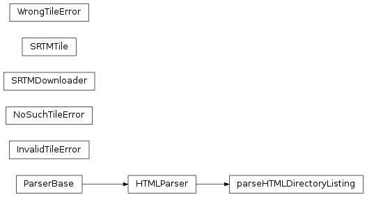
4   pylayers.gis.srtm Module

4.1   Classes

HTMLParser(*[, convert_charrefs])	Find tags and other markup and call handler functions.
InvalidTileError(lat, lon)	Raised when the SRTM tile file contains invalid data.
NoSuchTileError(lat, lon)	Raised when there is no tile for a region.
SRTMDownloader([server, directory, …])	Automatically download SRTM tiles.
SRTMTile(f, lat, lon)	Base class for all SRTM tiles.
WrongTileError(tile_lat, tile_lon, req_lat, …)	Raised when the value of a pixel outside the tile area is reque sted.
parseHTMLDirectoryListing()

4.2   Class Inheritance Diagram

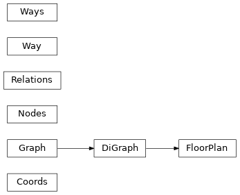
5   pylayers.gis.osmparser Module

Module OSMParser

5.1   Functions

buildingsparse(filename)	parse buildings
extract(alat, alon, fileosm, fileout)	extraction of an osm sub region using osmconvert
getbdg(fileosm[, verbose])	get building from osm file
getosm(**kwargs)	get osm region from osmapi
urlopen(url[, data, timeout, cafile, …])

5.2   Classes

Basemap([llcrnrlon, llcrnrlat, urcrnrlon, …])
Coords([idx, latlon])	Coords describes a set of points in OSM
FloorPlan(rootid, coords, nodes, ways, relations)	FloorPlan class derived from nx.DigGraph
Nodes	osm Nodes container
OsmApi([username, password, passwordfile, …])	Main class of osmapi, instanciate this class to use osmapi
PolyCollection(verts[, sizes, closed])
PyLayers	Generic PyLayers Meta Class
Relations
Way(refs, tags, coords)	A Way is a polyline or a Polygon (if closed)
Ways	Attributes ———-

5.3   Class Inheritance Diagram

6   pylayers.gis.ezone Module

6.1   Functions

arr2lp(arr)	convert zeros separated array to list of array
colorbar(mappable[, cax, ax])	Create a colorbar for a ScalarMappable instance.
conv(extent, m[, mode])	convert zone to cartesian or lon lat
ctrad2qt(extent)	convert center,radius into a list of qt regions
dectile([prefix])	decode tile name
distance_on_earth(lat1, long1, lat2, long2)	Compute great circle distance (the shortest distance over the earths surface) between 2 points on earth: A(lat1,lon1) and B(lat2,lon2)
dqt(ud16, lL0)	decode quad tree integer to lon Lat
enctile(lon, lat)	encode tile prefix from (lon,lat)
ent(lL)	encode lon Lat in natural integer
eqt(lL)	encode lon Lat in quad tree integer
expand(A)	expand numpy array
ext2qt([extent, lL0])	convert an extent region into a list of qt regions
get_google_elev_profile(node0, node1[, …])	return elevation profile between 2 nodes using google elevation API data
get_osm_elev_profile(node0, node1[, nb_samples])	return elevation profile between 2 nodes using google elevation API data
haversine(lat1, lon1, lat2, lon2[, mode])	lat 1 (Na) lon 1 (Na) lat 2 (Nb) lon 2 (Nb)
lL2ext(lL)	convert a lonLat into its qt extent
lab2ext(lab, lL0)	label to extent
make_axes_locatable(axes)
maxloc(f[, threshold])	determine local maximum above a threshold
minsec2dec(old)	convert latlon from DMS (minute second) to DD (decimal)
zone(pt[, rm])	extract a region from a point and a radius

6.2   Classes

Basemap([llcrnrlon, llcrnrlat, urcrnrlon, …])
DEM(prefix)	Class Digital Elevation Model
Ezone(prefix)	Earth zone
Polygon([shell, holes])	A two-dimensional figure bounded by a linear ring
PyLayers	Generic PyLayers Meta Class

6.3   Class Inheritance Diagram

7   pylayers.antprop.antenna Module

7.1   Functions

AFLegendre(N, M, x)	calculate Pmm1n and Pmp1n
AFLegendre2(L, M, x)	calculate Pmm1l and Pmp1l
AFLegendre3(L, M, x)	calculate Pmm1l and Pmp1l
BeamGauss(theta, phi[, Gmax, HPBW_az, …])	Beam with a Gaussian shape
CartToSphere(theta, phi, ex, ey, ez[, …])	Convert from Cartesian to Spherical
F0(nu, sigma)	F0 function for horn antenna pattern
F1(nu, sigma)	F1 function for horn antenna pattern
RepAzimuth1(Ec, theta, phi[, th, typ])	response in azimuth
SSHFunc(L, theta, phi)	ssh function
SSHFunc2(L, theta, phi)	ssh function version 2
VW(l, m, theta, phi)	evaluate vector Spherical Harmonics basis functions
VW0(n, m, x, phi, Pmm1n, Pmp1n)	evaluate vector Spherical Harmonics basis functions
VW2(l, m, x, phi, Pmm1l, Pmp1l)	evaluate vector Spherical Harmonics basis functions
cformat(x, y, **kwargs)	complex format
compdiag(k, A, th, ph, Fthr, Fphr[, typ, …])	makes comparison between original pattern and reconstructed pattern
cylinder(fig, pa, pb, R)	plot a cylinder
displot(pt, ph[, arrow])	discontinuous plot
factorial(*args, **kwds)	factorial is deprecated! Importing factorial from scipy.misc is deprecated in scipy 1.0.0.
forcesympol(A)	plot VSH transform vsh basis in 3D plot
index_vsh(L, M)	vector spherical harmonics indexing
indexssh(L[, mirror])	create [l,m] indexation from Lmax
indexvsh(L)	calculate index of vsh
level_energy(A, l[, ifreq, L])	calculates energy of the level l
lmreshape(coeff[, L])	level and mode reshaping
make_axes_locatable(axes)
modeMax(coeff[, L, ifreq])	calculates maximal mode
mode_energy(C, M[, L, ifreq])	calculates mode energy
mode_energy2(A, m[, ifreq, L])	calculates mode energy (version 2)
mulcplot(x, y, **kwargs)	handling multiple complex variable plots
plotVW(l, m, theta, phi[, sf])	plot VSH transform vsh basis in 3D plot
pol3D(fig, rho, theta, phi[, sf, shade, title])	polar 3D surface plot
polycol(lpoly[, var])	plot a collection of polygon
rc(group, **kwargs)	Set the current rc params.
rectplot(x, xpos[, ylim])	plot rectangles on an axis
relative_error(Eth_original, Eph_original, …)	calculate relative error between original and model
shadow(data, ax)	data : np.array 0 or 1 ax : matplotlib.axes
show3D(F, theta, phi, k[, col])	show 3D matplotlib diagram
ssh(A[, L, dsf])	Parameters ———-
sshModel(c, d[, L])	calculates sshModel
vsh(A[, dsf])	Parameters ———-
zeros(shape[, dtype, order])	Return a new array of given shape and type, filled with zeros.

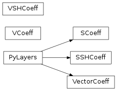
7.2   Classes

AntPosRot(name, p, T)	Antenna + position + Rotation
Antenna([typ])	Attributes ———-
FontProperties([family, style, variant, …])	A class for storing and manipulating font properties.
MaxNLocator(*args, **kwargs)	Select no more than N intervals at nice locations.
Pattern()	Class Pattern
PolyCollection(verts[, sizes, closed])
PyLayers	Generic PyLayers Meta Class
SCoeff([typ, fmin, fmax, lmax, data, dtype, …])	scalar Spherical Harmonics coefficients
SSHCoeff(Cx, Cy, Cz)	scalar spherical harmonics
VCoeff(typ[, fmin, fmax, data, dtype, ind, …])	Spherical Harmonics Coefficient
VSHCoeff(Br, Bi, Cr, Ci)	Vector Spherical Harmonics Coefficients class
VectorCoeff(typ[, fmin, fmax, data, dtype, …])	class vector spherical harmonics

7.3   Class Inheritance Diagram

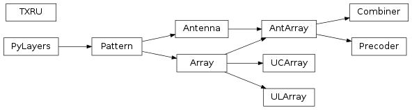
8   pylayers.antprop.aarray Module

8.1   Functions

k2xyz(ik, sh)	Parameters ———-
weights(nx, nz, kx, kz, Kx, Kz)	Practical Demonstration of Limited Feedback Beamforming for mmWave Systems
xyztok(iz, iy, ix[, Nx, Ny])

8.2   Classes

AntArray(**kwargs)	Class AntArray
Array(p[, w])	Array class
Combiner(Wbr, Whb, Wsh)
Precoder(Fhs, Fbh, Fht)
TXRU()	Tranceiver Units
UCArray(p[, w])	Uniform Circular Array
ULArray(**kwargs)	Uniform Linear Array

8.3   Class Inheritance Diagram

9   pylayers.antprop.spharm Module

9.1   Functions

AFLegendre(N, M, x)	calculate Pmm1n and Pmp1n
AFLegendre2(L, M, x)	calculate Pmm1l and Pmp1l
AFLegendre3(L, M, x)	calculate Pmm1l and Pmp1l
VW(l, m, theta, phi)	evaluate vector Spherical Harmonics basis functions
VW0(n, m, x, phi, Pmm1n, Pmp1n)	evaluate vector Spherical Harmonics basis functions
VW2(l, m, x, phi, Pmm1l, Pmp1l)	evaluate vector Spherical Harmonics basis functions
cformat(x, y, **kwargs)	complex format
cylinder(fig, pa, pb, R)	plot a cylinder
displot(pt, ph[, arrow])	discontinuous plot
factorial(*args, **kwds)	factorial is deprecated! Importing factorial from scipy.misc is deprecated in scipy 1.0.0.
index_vsh(L, M)	vector spherical harmonics indexing
indexssh(L[, mirror])	create [l,m] indexation from Lmax
indexvsh(L)	calculate index of vsh
mulcplot(x, y, **kwargs)	handling multiple complex variable plots
plotVW(l, m, theta, phi[, sf])	plot VSH transform vsh basis in 3D plot
pol3D(fig, rho, theta, phi[, sf, shade, title])	polar 3D surface plot
polycol(lpoly[, var])	plot a collection of polygon
rc(group, **kwargs)	Set the current rc params.
rectplot(x, xpos[, ylim])	plot rectangles on an axis
shadow(data, ax)	data : np.array 0 or 1 ax : matplotlib.axes

9.2   Classes

FontProperties([family, style, variant, …])	A class for storing and manipulating font properties.
PolyCollection(verts[, sizes, closed])
PyLayers	Generic PyLayers Meta Class
SCoeff([typ, fmin, fmax, lmax, data, dtype, …])	scalar Spherical Harmonics coefficients
SSHCoeff(Cx, Cy, Cz)	scalar spherical harmonics
VCoeff(typ[, fmin, fmax, data, dtype, ind, …])	Spherical Harmonics Coefficient
VSHCoeff(Br, Bi, Cr, Ci)	Vector Spherical Harmonics Coefficients class
VectorCoeff(typ[, fmin, fmax, data, dtype, …])	class vector spherical harmonics

9.3   Class Inheritance Diagram

10   pylayers.antprop.antssh Module

10.1   Functions

AFLegendre(N, M, x)	calculate Pmm1n and Pmp1n
AFLegendre2(L, M, x)	calculate Pmm1l and Pmp1l
AFLegendre3(L, M, x)	calculate Pmm1l and Pmp1l
CartToSphere(theta, phi, ex, ey, ez[, …])	Convert from Cartesian to Spherical
SSHFunc(L, theta, phi)	ssh function
SSHFunc2(L, theta, phi)	ssh function version 2
SphereToCart(theta, phi, eth, eph, bfreq)	Spherical to Cartesian
VW(l, m, theta, phi)	evaluate vector Spherical Harmonics basis functions
VW0(n, m, x, phi, Pmm1n, Pmp1n)	evaluate vector Spherical Harmonics basis functions
VW2(l, m, x, phi, Pmm1l, Pmp1l)	evaluate vector Spherical Harmonics basis functions
cformat(x, y, **kwargs)	complex format
cylinder(fig, pa, pb, R)	plot a cylinder
displot(pt, ph[, arrow])	discontinuous plot
factorial(*args, **kwds)	factorial is deprecated! Importing factorial from scipy.misc is deprecated in scipy 1.0.0.
index_vsh(L, M)	vector spherical harmonics indexing
indexssh(L[, mirror])	create [l,m] indexation from Lmax
indexvsh(L)	calculate index of vsh
mulcplot(x, y, **kwargs)	handling multiple complex variable plots
plotVW(l, m, theta, phi[, sf])	plot VSH transform vsh basis in 3D plot
pol3D(fig, rho, theta, phi[, sf, shade, title])	polar 3D surface plot
polycol(lpoly[, var])	plot a collection of polygon
rc(group, **kwargs)	Set the current rc params.
rectplot(x, xpos[, ylim])	plot rectangles on an axis
shadow(data, ax)	data : np.array 0 or 1 ax : matplotlib.axes
ssh(A[, L, dsf])	Parameters ———-
sshs(G, fGHz, th, ph[, L])	scalar spherical harmonics transform

11   pylayers.antprop.antvsh Module

11.1   Functions

AFLegendre(N, M, x)	calculate Pmm1n and Pmp1n
AFLegendre2(L, M, x)	calculate Pmm1l and Pmp1l
AFLegendre3(L, M, x)	calculate Pmm1l and Pmp1l
VW(l, m, theta, phi)	evaluate vector Spherical Harmonics basis functions
VW0(n, m, x, phi, Pmm1n, Pmp1n)	evaluate vector Spherical Harmonics basis functions
VW2(l, m, x, phi, Pmm1l, Pmp1l)	evaluate vector Spherical Harmonics basis functions
cformat(x, y, **kwargs)	complex format
cylinder(fig, pa, pb, R)	plot a cylinder
displot(pt, ph[, arrow])	discontinuous plot
factorial(*args, **kwds)	factorial is deprecated! Importing factorial from scipy.misc is deprecated in scipy 1.0.0.
index_vsh(L, M)	vector spherical harmonics indexing
indexssh(L[, mirror])	create [l,m] indexation from Lmax
indexvsh(L)	calculate index of vsh
mulcplot(x, y, **kwargs)	handling multiple complex variable plots
plotVW(l, m, theta, phi[, sf])	plot VSH transform vsh basis in 3D plot
pol3D(fig, rho, theta, phi[, sf, shade, title])	polar 3D surface plot
polycol(lpoly[, var])	plot a collection of polygon
rc(group, **kwargs)	Set the current rc params.
rectplot(x, xpos[, ylim])	plot rectangles on an axis
shadow(data, ax)	data : np.array 0 or 1 ax : matplotlib.axes
vsh(A[, dsf])	Parameters ———-

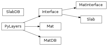
12   pylayers.antprop.slab Module

12.1   Functions

calRT_3layers_model(x, epsr, d, fGHz, theta)	calculate R and T for an homogeneous Slab
calRT_homogeneous_model(x, epsr, d, fGHz, theta)	calculate R and T for an homogeneous Slab
calsig(cval, fGHz[, typ])	evaluate sigma from epsr or index at a given frequency

12.2   Classes

Interface([fGHz, theta, name])	Interface between 2 medium
Mat(name, **dm)	Handle constitutive materials dictionnary
MatDB([_fileini, dm])	MatDB Class : Material database
MatInterface(lmat, l, fGHz, theta)	MatInterface : Class for Interface between two materials
PyLayers	Generic PyLayers Meta Class
Slab(name, matDB[, ds])	Handle a Slab
SlabDB([fileslab, filemat, ds, dm])	Slab data base
interp1d(x, y[, kind, axis, copy, …])	Interpolate a 1-D function.

12.3   Class Inheritance Diagram

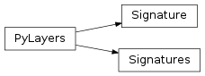
13   pylayers.antprop.signature Module

13.1   Functions

gidl(g)	gi without diffraction
plot_lines(ax, ob[, color])	plot lines with colors
plot_poly(ax, ob[, color])	plot polygon
shLtmp(L)
showsig(L, s[, tx, rx])	show signature
showsig2(lsig, L, tahe)
valid(lsig, L[, tahe])	Check if a signature is valid.

13.2   Classes

Axes3D(fig[, rect])	3D axes object.
PyLayers	Generic PyLayers Meta Class
Rays(pTx, pRx)	Class handling a set of rays
Signature(sig)	class Signature
Signatures(L, source, target[, cutoff, …])	set of Signature given 2 Gt cycle (convex) indices
tqdm([iterable, desc, total, leave, file, …])	Decorate an iterable object, returning an iterator which acts exactly like the original iterable, but prints a dynamically updating progressbar every time a value is requested.

13.3   Class Inheritance Diagram

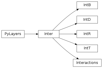
14   pylayers.antprop.interactions Module

14.1   Classes

IntB([data, dtype, idx, slab])	Local Basis interaction class
IntD([data, dtype, idx, fGHz, slab])	diffraction interaction class
IntR([data, dtype, idx, slab])	Reflexion interaction class
IntT([data, dtype, idx, slab])	Transmission interaction class
Inter([typ, data, dtype, idx, _filemat, …])	Interactions
Interactions([slab])	Interaction parameters
Interface([fGHz, theta, name])	Interface between 2 medium
Mat(name, **dm)	Handle constitutive materials dictionnary
MatDB([_fileini, dm])	MatDB Class : Material database
MatInterface(lmat, l, fGHz, theta)	MatInterface : Class for Interface between two materials
PyLayers	Generic PyLayers Meta Class
Slab(name, matDB[, ds])	Handle a Slab
SlabDB([fileslab, filemat, ds, dm])	Slab data base
interp1d(x, y[, kind, axis, copy, …])	Interpolate a 1-D function.

14.2   Class Inheritance Diagram

15   pylayers.antprop.diffraction Module

15.1   Functions

diff(fGHz, phi0, phi, si, sd, N, beta)

diffraction coefficient

16   pylayers.antprop.diffRT Module

16.1   Functions

Dfunc(sign, k, N, dphi, si, sd[, xF, F, beta])	Parameters ———-
FreF(x)	F function from Pathack
FreF2(x)	F function using numpy fresnel function
FresnelI(x)	calculates Fresnel integral
G(N, phi0, Ro, Rn)	grazing angle correction
R(th, k, er, err, sigma, ur, urr, deltah)	R coeff
diff(fGHz, phi0, phi, si, sd, N, mat0, matN)	Luebbers Diffration coefficient for Ray tracing

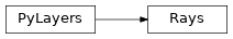
17   pylayers.antprop.rays Module

17.1   Classes

Ctilde()	container for the 4 components of the polarimetric ray channel
IntB([data, dtype, idx, slab])	Local Basis interaction class
IntD([data, dtype, idx, fGHz, slab])	diffraction interaction class
IntR([data, dtype, idx, slab])	Reflexion interaction class
IntT([data, dtype, idx, slab])	Transmission interaction class
Inter([typ, data, dtype, idx, _filemat, …])	Interactions
Interactions([slab])	Interaction parameters
Interface([fGHz, theta, name])	Interface between 2 medium
Layout([arg])	Handling Layout
Mat(name, **dm)	Handle constitutive materials dictionnary
MatDB([_fileini, dm])	MatDB Class : Material database
MatInterface(lmat, l, fGHz, theta)	MatInterface : Class for Interface between two materials
PyLayers	Generic PyLayers Meta Class
Rays(pTx, pRx)	Class handling a set of rays
Slab(name, matDB[, ds])	Handle a Slab
SlabDB([fileslab, filemat, ds, dm])	Slab data base
interp1d(x, y[, kind, axis, copy, …])	Interpolate a 1-D function.

17.2   Class Inheritance Diagram

18   pylayers.antprop.loss Module

18.1   Functions

Dgrid_points(points, Px)	distance point to grid
Dgrid_zone(zone, Px)	Distance point to zone
FMetisShad(fGHz, r, D[, sign])	F Metis shadowing function
FMetisShad2(fGHz, r, D[, sign])	F Metis shadowing function
Loss0(S, rx, ry, f, p)	calculate Loss through Layers for theta=0 deg
LossMetisShadowing(fGHz, tx, rx, pg, uw, uh, …)	Calculate the Loss from
LossMetisShadowing2(fGHz, tx, rx, pg, uw, …)	Calculate the Loss from
Loss_diff(u)	calculate Path Loss of the diffraction
Losst(L, fGHz, p1, p2[, dB, bceilfloor])	calculate Losses between links p1-p2
OneSlopeMdl(D, n, fGHz)	one slope model
PL(fGHz, pts, p[, n, dB, d0])	calculate Free Space Path Loss
PL0(fGHz[, GtdB, GrdB, R])	Path Loss at frequency fGHZ @ R
bullington(d, height, fGHz)	edges attenuation with Bullington method
calnu(h, d1, d2, fGHz)	Calculate the diffraction Fresnel parameter
cdf(x[, colsym, lab, lw])	plot the cumulative density function
cost2100(pMS, pBS, fGHz[, nfloor, dB])	cost 2100 model
cost231(pBS, pMS, hroof, phir, wr, fMHz[, …])	Walfish Ikegami model (COST 231)
cost259(pMS, pBS, fMHz)	cost259 model
cover(X, Y, Z, Ha, Hb, fGHz, K[, method])	outdoor coverage on a region
deygout(d, height, fGHz, L, depth)	Deygout attenuation
gaspl(d, fGHz, T, PhPa, wvden)	attenuation due to atmospheric gases
hata(pMS, pBS, fGHz, hMS, hBS, typ)	Hata Path loss model
jit([signature_or_function, locals, target, …])	This decorator is used to compile a Python function into native code.
lossref_compute(P, h0, h1[, k])	compute loss and reflection rays on curved earth
route(X, Y, Z, Ha, Hb, fGHz, K[, method])	diffraction loss along a route
two_rays_curvedearthold(P, h0, h1[, fGHz])	Parameters ———-
two_rays_flatearth(fGHz, **kwargs)	Parameters ———-
visuPts(S, nu, nd, Pts, Values[, fig, sp, …])	visuPt : Visualization of values a given points

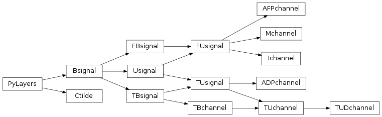
19   pylayers.antprop.channel Module

19.1   Classes

ADPchannel([x, dtype, y, dtype, az, dtype, …])	Angular Delay Profile channel
AFPchannel([x, dtype, y, dtype, tx, dtype, …])	Angular Frequency Profile channel
Axes3D(fig[, rect])	3D axes object.
Ctilde()	container for the 4 components of the polarimetric ray channel
Mchannel(x, y, **kwargs)	Handle the measured channel
PyLayers	Generic PyLayers Meta Class
TBchannel([x, dtype, y, dtype, label])	radio channel in non uniform delay domain
TUDchannel([x, dtype, y, dtype, taud, …])	Uniform channel in Time domain with delay
TUchannel([x, dtype, y, dtype, label])	Uniform channel in delay domain
Tchannel([x, y, tau, shape, dtype, dod, …])	Handle the transmission channel

19.2   Class Inheritance Diagram

20   pylayers.antprop.loss Module

20.1   Functions

Dgrid_points(points, Px)	distance point to grid
Dgrid_zone(zone, Px)	Distance point to zone
FMetisShad(fGHz, r, D[, sign])	F Metis shadowing function
FMetisShad2(fGHz, r, D[, sign])	F Metis shadowing function
Loss0(S, rx, ry, f, p)	calculate Loss through Layers for theta=0 deg
LossMetisShadowing(fGHz, tx, rx, pg, uw, uh, …)	Calculate the Loss from
LossMetisShadowing2(fGHz, tx, rx, pg, uw, …)	Calculate the Loss from
Loss_diff(u)	calculate Path Loss of the diffraction
Losst(L, fGHz, p1, p2[, dB, bceilfloor])	calculate Losses between links p1-p2
OneSlopeMdl(D, n, fGHz)	one slope model
PL(fGHz, pts, p[, n, dB, d0])	calculate Free Space Path Loss
PL0(fGHz[, GtdB, GrdB, R])	Path Loss at frequency fGHZ @ R
bullington(d, height, fGHz)	edges attenuation with Bullington method
calnu(h, d1, d2, fGHz)	Calculate the diffraction Fresnel parameter
cdf(x[, colsym, lab, lw])	plot the cumulative density function
cost2100(pMS, pBS, fGHz[, nfloor, dB])	cost 2100 model
cost231(pBS, pMS, hroof, phir, wr, fMHz[, …])	Walfish Ikegami model (COST 231)
cost259(pMS, pBS, fMHz)	cost259 model
cover(X, Y, Z, Ha, Hb, fGHz, K[, method])	outdoor coverage on a region
deygout(d, height, fGHz, L, depth)	Deygout attenuation
gaspl(d, fGHz, T, PhPa, wvden)	attenuation due to atmospheric gases
hata(pMS, pBS, fGHz, hMS, hBS, typ)	Hata Path loss model
jit([signature_or_function, locals, target, …])	This decorator is used to compile a Python function into native code.
lossref_compute(P, h0, h1[, k])	compute loss and reflection rays on curved earth
route(X, Y, Z, Ha, Hb, fGHz, K[, method])	diffraction loss along a route
two_rays_curvedearthold(P, h0, h1[, fGHz])	Parameters ———-
two_rays_flatearth(fGHz, **kwargs)	Parameters ———-
visuPts(S, nu, nd, Pts, Values[, fig, sp, …])	visuPt : Visualization of values a given points

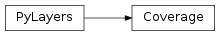
21   pylayers.antprop.coverage Module

21.1   Classes

CheckButtons(ax, labels, actives)	A GUI neutral radio button.
Coverage([_fileini])	Handle Layout Coverage
Layout([arg])	Handling Layout
PyLayers	Generic PyLayers Meta Class
RadioNode([name, typ, _fileini, _fileant])	container for a Radio Node
Slider(ax, label, valmin, valmax[, valinit, …])	A slider representing a floating point range.
Trajectories()	Define a list of trajectory
Trajectory([df, ID, name, typ])	define a trajectory
datetime(year, month, day[, hour[, minute[, …)	The year, month and day arguments are required.
product	product(*iterables, repeat=1) –> product object

21.2   Class Inheritance Diagram

22   pylayers.antprop.coeffModel Module

22.1   Functions

RepAzimuth1(Ec, theta, phi[, th, typ])	response in azimuth
level_energy(A, l[, ifreq, L])	calculates energy of the level l
lmreshape(coeff[, L])	level and mode reshaping
modeMax(coeff[, L, ifreq])	calculates maximal mode
mode_energy(C, M[, L, ifreq])	calculates mode energy
mode_energy2(A, m[, ifreq, L])	calculates mode energy (version 2)
relative_error(Eth_original, Eph_original, …)	calculate relative error between original and model
sshModel(c, d[, L])	calculates sshModel
zeros(shape[, dtype, order])	Return a new array of given shape and type, filled with zeros.

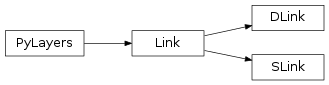
23   pylayers.simul.link Module

23.1   Classes

AFPchannel([x, dtype, y, dtype, tx, dtype, …])	Angular Frequency Profile channel
Antenna([typ])	Attributes ———-
Ctilde()	container for the 4 components of the polarimetric ray channel
DLink(**kwargs)	Deterministic Link Class
Layout([arg])	Handling Layout
Link()	Link class
PyLayers	Generic PyLayers Meta Class
RadioNode([name, typ, _fileini, _fileant])	container for a Radio Node
Rays(pTx, pRx)	Class handling a set of rays
SLink()
Signature(sig)	class Signature
Signatures(L, source, target[, cutoff, …])	set of Signature given 2 Gt cycle (convex) indices
Tchannel([x, y, tau, shape, dtype, dod, …])	Handle the transmission channel
VTKDataSource	This source manages a VTK dataset given to it.

23.2   Class Inheritance Diagram

24   pylayers.simul.exploit Module

24.1   Classes

Axes3D(fig[, rect])	3D axes object.
Bsignal([x, dtype, y, dtype, label])	Signal with an embedded time base
Error
Exploit([simnetfile])	class Exploit
FBsignal([x, dtype, y, dtype, label])	FBsignal : Base signal in Frequency domain
FHsignal([x, dtype, y, dtype, label])	FHsignal : Hermitian uniform signal in Frequency domain
FUsignal([x, dtype, y, dtype, label])	FUsignal : Uniform signal in Frequency Domain
Noise([ti, tf, fsGHz, PSDdBmpHz, NF, R, seed])	Create noise
PolyCollection(verts[, sizes, closed])
PyLayers	Generic PyLayers Meta Class
TBsignal([x, dtype, y, dtype, label])	Based signal in Time domain
TUsignal([x, dtype, y, dtype, label])	Uniform signal in time domain
Usignal([x, dtype, y, dtype, label])	Signal with an embedded uniform Base

24.2   Class Inheritance Diagram

25   pylayers.simul.exploit_simulnet Module

25.1   Classes

exploit([filename])

This class is for exploitation of simulnet output

25.2   Class Inheritance Diagram

26   pylayers.simul.simulnet Module

26.1   Classes

Agent(**args)	Class Agent
CheckButtons(ax, labels, actives)	A GUI neutral radio button.
EMSolver([L])	Invoque an electromagnetic solver
Gcom(net, sim)	Communication graph
Layout([arg])	Handling Layout
Network([owner, EMS, PN])	Network class
Node(**kwargs)	Class Node
PNetwork(**args)	Process version of the Network class
Process(env, generator)	Process an event yielding generator.
PyLayers	Generic PyLayers Meta Class
Save(**args)	Save all variables of a simulnet simulation.
ShowNet(**args)	Show network process
ShowTable(**args)	Show table process
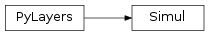
Simul()	Attributes ———-
Slab(name, matDB[, ds])	Handle a Slab
Slider(ax, label, valmin, valmax[, valinit, …])	A slider representing a floating point range.
Trajectories()	Define a list of trajectory
Trajectory([df, ID, name, typ])	define a trajectory
datetime(year, month, day[, hour[, minute[, …)	The year, month and day arguments are required.

26.2   Class Inheritance Diagram

27   pylayers.simul.simultraj Module

27.1   Classes

AFPchannel([x, dtype, y, dtype, tx, dtype, …])	Angular Frequency Profile channel
Antenna([typ])	Attributes ———-
Axes3D(fig[, rect])	3D axes object.
Basemap([llcrnrlon, llcrnrlat, urcrnrlon, …])
Body([_filebody, _filemocap, _filewear, …])	Class to manage a Body model
Button(ax, label[, image, color, hovercolor])	A GUI neutral button.
CheckButtons(ax, labels, actives)	A GUI neutral radio button.
CorSer([serie, day, source, layout])	Handle CORMORAN measurement data
Ctilde()	container for the 4 components of the polarimetric ray channel
Cursor(ax[, horizOn, vertOn, useblit])	A horizontal and vertical line that spans the axes and moves with the pointer.
DF([b, a])	Digital Filter Class
DLink(**kwargs)	Deterministic Link Class
Device([devname, ID, owner, typ])	Device Class
Layout([arg])	Handling Layout
Link()	Link class
Network([owner, EMS, PN])	Network class
Pool	alias of pathos.multiprocessing.ProcessPool
PyLayers	Generic PyLayers Meta Class
RadioNode([name, typ, _fileini, _fileant])	container for a Radio Node
Rays(pTx, pRx)	Class handling a set of rays
SLink()
SelectL(L, fig, ax)	Associates a Layout and a figure
Signature(sig)	class Signature
Signatures(L, source, target[, cutoff, …])	set of Signature given 2 Gt cycle (convex) indices
Simul([source, verbose])	Link oriented simulation
Slider(ax, label, valmin, valmax[, valinit, …])	A slider representing a floating point range.
Tchannel([x, y, tau, shape, dtype, dod, …])	Handle the transmission channel
VTKDataSource	This source manages a VTK dataset given to it.
combinations	combinations(iterable, r) –> combinations object
partial	partial(func, *args, **keywords) - new function with partial application of the given arguments and keywords.
product	product(*iterables, repeat=1) –> product object

27.2   Class Inheritance Diagram

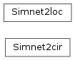
28   pylayers.exploit.simnet Module

28.1   Classes

Simnet2cir([simnetfile])	This class allows to perform a raytracing simulation from a simulnet simulation.
Simnet2loc([savefile])	Summary ——-

28.2   Class Inheritance Diagram

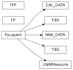
29   pylayers.measures.mesuwb Module

29.1   RAW_DATA Class

RAW_DATA.__init__(d)

Initialize self.

29.2   CAL_DATA Class

CAL_DATA.__init__(d)	depending of the version of scipy io.loadma do not give the same output
CAL_DATA.plot()
CAL_DATA.getwave()

29.3   Fdd Class

Fdd.__init__(d)
Fdd.plot([typ])	plot Fdd

29.4   Tdd Class

Tdd.__init__(d)	Initialize self.
Tdd.PL(fmin, fmax, B)	Calculate NB Path Loss on a given UWB frequency band
Tdd.show([fig, delay, display, title, col, …])	show the 4 Impulse Radio Impulse responses
Tdd.show_span([delay, wide])	show span
Tdd.box()	evaluate min and max of the 4 channels
Tdd.plot([type])	type : raw | filter

29.5   TFP Class

TFP.__init__()	Initialize self.
TFP.append(FP)	append data to fingerprint

29.6   FP Class

FP.__init__(M, k[, alpha, Tint, sym, nint, …])

object constructor

29.7   UWBMeasure

UWBMeasure.__init__([nTx, h, display])	object constructor
UWBMeasure.info()
UWBMeasure.show([fig, delay, display, col, …])	show measurement in time domain
UWBMeasure.Epercent()
UWBMeasure.toa_max2()	calculate toa_max (meth2)
UWBMeasure.tau_Emax()	calculate the delay of energy peak
UWBMeasure.tau_moy([display])	calculate mean excess delay
UWBMeasure.tau_rms([display])	calculate the rms delay spread
UWBMeasure.toa_new([display])	descendant threshold based toa estimation
UWBMeasure.toa_win([n, display])	descendant threshold based toa estimation
UWBMeasure.toa_max([n, display])	descendant threshold based toa estimation
UWBMeasure.toa_th(r, k[, display])	threshold based toa estimation using energy peak
UWBMeasure.toa_cum(n[, display])	threshold based toa estimation using cumulative energy
UWBMeasure.taumax()
UWBMeasure.Emax([Tint, sym, dB])	calculate maximum energy
UWBMeasure.Etot([toffns, tdns, dB])	Calculate total energy for the 4 channels
UWBMeasure.Efirst([Tint, sym, dB])	calculate energy in first path
UWBMeasure.Etau0([Tint, sym, dB])	calculate the energy around delay tau0
UWBMeasure.ecdf([Tnoise, rem_noise, …])	calculate energy cumulative density function
UWBMeasure.tdelay()	build an array with delay values
UWBMeasure.fp([alpha])	build fingerprint
UWBMeasure.outlatex(S)	measurement output latex

29.8   Utility Functions

mesname(n, dirname[, h])	get the measurement data filename
ptw1()	return W1 Tx and Rx points
visibility()	determine visibility type of WHERE1 measurements campaign points
trait(filename[, itx, dtype, dico, h])	evaluate various parameters for all measures in itx array

29.9   Functions

linspace(start, stop[, num, endpoint, …])	Return evenly spaced numbers over a specified interval.
mesname(n, dirname[, h])	get the measurement data filename
polyfit(x, y, deg[, rcond, full, w, cov])	Least squares polynomial fit.
polyval(p, x)	Evaluate a polynomial at specific values.
ptw1()	return W1 Tx and Rx points
trait(filename[, itx, dtype, dico, h])	evaluate various parameters for all measures in itx array
visibility()	determine visibility type of WHERE1 measurements campaign points

29.10   Classes

CAL_DATA(d)	ch1 ch2 ch3 ch4 vna_att1 vna_att2 vna_freq
FP(M, k[, alpha, Tint, sym, nint, thlos, …])	Fingerprint class
Fdd(d)	Frequency Domain Deconv Data
PyLayers	Generic PyLayers Meta Class
RAW_DATA(d)	Members ——- ch1 ch2 ch3 ch4 time timeTX tx
TFP()	Tx Rx distance los_cond
Tdd(d)	Time Domain Deconv Data
UWBMeasure([nTx, h, display])	UWBMeasure class

29.11   Class Inheritance Diagram

30   pylayers.measures.mesmimo Module

30.1   Classes

ADPchannel([x, dtype, y, dtype, az, dtype, …])	Angular Delay Profile channel
AFPchannel([x, dtype, y, dtype, tx, dtype, …])	Angular Frequency Profile channel
AntArray(**kwargs)	Class AntArray
Array(p[, w])	Array class
Axes3D(fig[, rect])	3D axes object.
Bsignal([x, dtype, y, dtype, label])	Signal with an embedded time base
BuiltinFunctionType	alias of builtins.builtin_function_or_method
BuiltinMethodType	alias of builtins.builtin_function_or_method
CodeType	alias of builtins.code
Combiner(Wbr, Whb, Wsh)
CoroutineType	alias of builtins.coroutine
Ctilde()	container for the 4 components of the polarimetric ray channel
DynamicClassAttribute([fget, fset, fdel, doc])	Route attribute access on a class to __getattr__.
Error
FBsignal([x, dtype, y, dtype, label])	FBsignal : Base signal in Frequency domain
FHsignal([x, dtype, y, dtype, label])	FHsignal : Hermitian uniform signal in Frequency domain
FUsignal([x, dtype, y, dtype, label])	FUsignal : Uniform signal in Frequency Domain
FrameType	alias of builtins.frame
FunctionType	alias of builtins.function
GeneratorType	alias of builtins.generator
GetSetDescriptorType	alias of builtins.getset_descriptor
LambdaType	alias of builtins.function
Layout([arg])	Handling Layout
MIMO(**kwargs)	This class handles the data coming from a MIMO Channel Sounder
MappingProxyType	alias of builtins.mappingproxy
Mchannel(x, y, **kwargs)	Handle the measured channel
MemberDescriptorType	alias of builtins.member_descriptor
Mesh5([_filename])	Class handling hdf5 measurement files
MethodType	alias of builtins.method
ModuleType	alias of builtins.module
Noise([ti, tf, fsGHz, PSDdBmpHz, NF, R, seed])	Create noise
PolyCollection(verts[, sizes, closed])
Precoder(Fhs, Fbh, Fht)
PyLayers	Generic PyLayers Meta Class
SCPI([port, timeout, verbose, Nr, Nt, emulated])
SimpleNamespace	A simple attribute-based namespace.
TBchannel([x, dtype, y, dtype, label])	radio channel in non uniform delay domain
TBsignal([x, dtype, y, dtype, label])	Based signal in Time domain
TUDchannel([x, dtype, y, dtype, taud, …])	Uniform channel in Time domain with delay
TUchannel([x, dtype, y, dtype, label])	Uniform channel in delay domain
TUsignal([x, dtype, y, dtype, label])	Uniform signal in time domain
TXRU()	Tranceiver Units
Tchannel([x, y, tau, shape, dtype, dod, …])	Handle the transmission channel
TracebackType	alias of builtins.traceback
UCArray(p[, w])	Uniform Circular Array
ULArray(**kwargs)	Uniform Linear Array
Usignal([x, dtype, y, dtype, label])	Signal with an embedded uniform Base
VLayout

30.2   Class Inheritance Diagram

31   pylayers.measures.cormoran Module

This module handles CORMORAN measurement data

31.1   CorSer Class

class pylayers.measures.cormoran.CorSer(serie=6, day=11, source='CITI', layout=False)

Handle CORMORAN measurement data

Hikob data handling from CORMORAN measurement campaign

11/06/2014

single subject (Bernard and Nicolas)

12/06/2014

several subject (Jihad, Eric , Nicolas)

align(devdf, hkbdf)

DEPRECATED align time of 2 data frames:

the time delta of the second data frame is applyied on the first one (e.g. time for devdf donwsampled by hkb data frame time)

devdf : device dataframe hkbdf : hkbdataframe

devdfc :

aligned copy device dataframe

hkbdfc :

aligned copy hkbdataframe

>>> from pylayers.measures.cormoran import *
>>> S=CorSer(6)
>>> devdf = S.devdf[S.devdf['id']=='HKB:15']
>>> hkbdf = S.hkb['AP1-AnkleLeft']
>>> devdf2,hkbdf2 = S.align(devdf,hkbdf)

animhkb(a, b, interval=10, save=False)

a : node name |number b : node name | number save : bool

animhkbAP(a, AP_list, interval=1, save=False, **kwargs)

a : node name AP_nb=[] save : bool

>>> from pylayers.measures.cormoran import *
>>> S = CorSer(6)
>>> S.animhkbAP('TorsoTopLeft',['AP1','AP2','AP3','AP4'],interval=100,xstart=58,figsize=(20,2))

ant

display device techno, id , id on body, body owner,…

compute_visibility(techno='HKB', square_mda=True, all_links=True)

determine visibility of links for a given techno

techno string

select the given radio technology of the nodes to determine

the visibility matrix

square_mda boolean

select ouput format

True : (device x device x timestamp) False : (link x timestamp)

all_links : bool

compute all links or just those for which data is available

if square_mda = True

intersection : (ndevice x nbdevice x nb_timestamp)

matrice of intersection (1 if link is cut 0 otherwise)

links : (nbdevice)

name of the links

if square_mda = False

intersection : (nblink x nb_timestamp)

matrice of intersection (1 if link is cut 0 otherwise)

links : (nblink x2)

name of the links

>>> from pylayers.measures.cormoran import *
>>> import matplotlib.pyplot as plt
>>> C=CorSer(serie=14,day=12)
>>> inter,links=C.compute_visibility(techno='TCR',square_mda=True)
>>> inter.shape
    (15, 15, 12473)
>>>C.imshowvisibility_i(inter,links)

dev

display device techno, id , id on body, body owner,…

devmapper(a, techno='')

retrieve name of device if input is number

or retrieve number of device if input is name

a : str | int

name |id |bodyid

techno : str

radio techno

a : string

dev name

ia : int

dev number

ba : string

dev refernce in body

subject : string

body owning the device

export_csv(**kwargs)

export to csv devices positions

unit : string (‘mm’|’cm’|’m’),

unit of positions in csv(default mm)

tunit: string

time unit in csv (default ‘ns’)

‘alias’: dict

dictionnary to replace name of the devices into the csv . example : if you want to replace a device id named ‘TCR:34’ to an id = 5, you have to add an entry in the alias dictionnary as : alias.update({‘TCR34’:5})

offset : np.array

apply an offset on positions

a csv file into the folder <PylayersProject>/netsave

getdevp(a, techno='', t='', fId='')

get a device position

a : str | int

name |id

techno : str

radio techno

optional :

t : float | list

given time |[time_start,time_stop]

pa : np.array()

>>> from pylayers.measures.cormoran import *
>>> S=CorSer(serie=34)
>>> a=S.getdevp('AP1','WristLeft')

getlink(a, b, techno='', t='')

get a link value

a : str | int

name |id

b : str | int

name |id

optional :

techno : str

radio techno

t : float | list

given time or [start,stop] time

Pandas Serie

>>> from pylayers.measures.cormoran import *
>>> S=CorSer(serie=34)
>>> S.getlink('AP1','WristLeft')

getlinkd(a, b, techno='', t='')

get the distance for a link between devices

a : str | int

name |id

b : str | int

name |id

optional

techno : str

radio techno

t : float | list

given time or [start,stop] time

dist : np.array()

all distances for all timestamps for the given link

>>> from pylayers.measures.cormoran import *
>>> S = CorSer(serie=6)
>>> d = S.getlinkd('AP1','WristLeft',techno='HKB')

getlinkp(a, b, technoa='', technob='', t='', fId='')

get a link devices positions

a : str | int

name |id

b : str | int

name |id

optional :

technoa : str

radio techno

technob : str

radio techno

t : float | list

given time | [time_start,time_stop]

OR

fId : int

frame id

pa,pb : np.array()

>>> from pylayers.measures.cormoran import *
>>> S=CorSer(serie=34)
>>> a,b=S.getlinkp('AP1','WristLeft')

imshow(time=100, kind='time')

DEPRECATED

kind : string

‘mean’,’std’

imshowvisibility(techno='HKB', t=0, **kwargs)

imshow visibility mda

techno : (HKB|TCR) t : float

time in second

>>> from pylayers.measures.cormoran import *
>>> import matplotlib.pyplot as plt
>>> C=CorSer(serie=6,day=12)
>>> inter,links=C.compute_visibility(techno='TCR',square_mda=True)
>>> i,l=C.imshowvisibility_i(inter,links)

pylayers.measures.CorSer.compute_visibility()

imshowvisibility_i(techno='HKB', t=0, **kwargs)

imshow visibility mda interactive

inter : (nb link x nb link x timestamps) links : (nblinks) time : intial time (s)

>>> from pylayers.measures.cormoran import *
>>> import matplotlib.pyplot as plt
>>> C=CorSer(serie=6,day=12)
>>> inter,links=C.visimda(techno='TCR',square_mda=True)
>>> i,l=C.imshowvisibility_i(inter,links)

lk2nd(lk)

transcode a lk from Id to real name

lk : string

>>> C=Corser(6)
>>> lk = 'HKB:15-HKB:7'
>>> C.lk2nd(lk)

loadlog()

load in self.log the log of the current serie from MeasurementLog.csv

mtlbsave()

Matlab format save

S{day}_{serie}

node_name node_place node_coord

HKB.{linkname}.tr HKB.{linkname}.rssi HKB.{linkname}.td HKB.{linkname}.dist HKB.{linkname}.sh HKB.{linkname}.dsh

TCR.{linkname}.tr HKB.{linkname}.range HKB.{linkname}.td HKB.{linkname}.dist HKB.{linkname}.sh

offset_setter(a='HKB:1', b='HKB:12', techno='', **kwargs)

offset setter

offset_setter_video(a='AP1', b='WristRight', **kwargs)

video offset setter

plot(a, b, techno='', t='', **kwargs)

ploting

a : str | int

name |id

b : str | int

name |id

techno : str (optional)

radio techno

t : float | list (optional)

given time or [start,stop] time

color : color distance : boolean (False)

plot distance instead of value

lin : boolean (False)

display linear value instead of dB

sqrtinv : boolean (False)

apply : “sqrt (1/ dataset)”

xoffset : float (0)

add an offset on x axis

yoffset : float (1|1e3|1e6)

add an offset on y axis

title : boolean (True)

display title

shortlabel : boolean (True)

enable short labelling

fontsize : int (18)

font size

returnlines : boolean

if True return the matplotlib ploted lines

>>> from pylayers.measures.cormoran import *
>>> S = CorSer(6)
>>> f,ax = S.plot('AP1','TorsoTopLeft',techno='HKB')
>>> f,ax = S.pltvisi('AP1','TorsoTopLeft',techno='HKB',fig=f,ax=ax)
>>> #f,ax = S.pltmob(fig=f,ax=ax)
>>> #plt.title('hatch = visibility / gray= mobility')
>>> plt.show()

pltgt(a, b, **kwargs)

plt ground truth

t0 t1 fig ax figsize: tuple linestyle’ inverse :False,

display 1/distance instead of distance

log : boolean

display log for distance intead of distance

gammma’:1.,

mulitplication factor for log : gamma*log(distance) this can be used to fit RSS

mode : string

‘HKB’ | ‘TCR’ | ‘FULL’

visi : boolean,

display visibility

color: string color (‘k’|’m’|’g’),

color to display the visibility area

hatch’: strin hatch type (‘//’)

hatch type to hatch visibility area

fontsize: int

title fontsize

>>> from pylayers.measures.cormoran import *
>>> S=CorSer(6)
>>> S.pltgt('AP1','TorsoTopLeft')

plthkb(a, b, techno='HKB', **kwargs)

plot Hikob devices

DEPRECATED

a : node name |number b : node name | number t0 : start time t1 : stop time

>>> from pylayers.measures.cormoran import *
>>> S = CorSer(6)
>>> f,ax = S.plthkb('AP1','TorsoTopLeft',techno='HKB')
>>> f,ax = S.pltvisi('AP1','TorsoTopLeft',techno='HKB',fig=f,ax=ax)
>>> f,ax = S.pltmob(fig=f,ax=ax)
>>> plt.title('hatch = visibility / gray= mobility')
>>> plt.show()

pltlk(a, b, **kwargs)

plot links

a : string

node a name

b : string

node b name

display: list

techno to be displayed

figsize t0: float

time start

t1 : float

time stop

colhk: plt.color

color of hk curve

colhk2:plt.color

color of hk curve2 ( if recirpocal)

linestylehk:

linestyle hk

coltcr:

color tcr curve

coltcr2:

color of tcr curve2 ( if recirpocal)

linestyletcr:

linestyle tcr

colgt:

color ground truth

inversegt:

invert ground truth

loggt: bool

apply a log10 factor to ground truth

gammagt:

applly a gamma factor to ground truth (if loggt ! )

fontsize:

font size of legend

visi:

display visibility indicator

axs :

list of matplotlib axes

>>> from pylayers.measures.cormoran import *
>>> S=CorSer(6)
>>> S.pltlk('AP1','TorsoTopLeft')

pltmob(**kwargs)

plot mobility

subject: str

subject to display () if ‘’, take the fist one from self.subject)

showvel : boolean

display filtered velocity

velth: float (0.7)

velocity threshold

fo : int (5)

filter order

fw: float (0.02)

0 < fw < 1 (fN <=> 1)

time_offset : int

add time_offset to start later

>>> from pylayers.measures.cormoran import *
>>> S = CorSer(6)
>>> f,ax = S.plthkb('AP1','TorsoTopLeft',techno='HKB')
>>> #f,ax = S.pltvisi('AP1','TorsoTopLeft',techno='HKB',fig=f,ax=ax)
>>> f,ax = S.pltmob(fig=f,ax=ax)
>>> plt.title('hatch = visibility / gray= mobility')
>>> plt.show()

plttcr(a, b, **kwargs)

plot TCR devices

a : node name |number b : node name | number t0 : start time t1 : stop time

pltvisi(a, b, techno='', **kwargs)

plot visibility between link a and b

color:

fill color

hatch:

hatch type

label_pos: (‘top’|’bottom’|’‘)

postion of the label

label_pos_off: float

offset of postion of the label

label_mob: str

prefix of label in mobility

label_stat: str

prefix of label static

>>> from pylayers.measures.cormoran import *
>>> S = CorSer(6)
>>> f,ax = S.plthkb('AP1','TorsoTopLeft',techno='HKB')
>>> f,ax = S.pltvisi('AP1','TorsoTopLeft',techno='HKB',fig=f,ax=ax)
>>> f,ax = S.pltmob(fig=f,ax=ax)
>>> plt.title('hatch = visibility / gray= mobility')
>>> plt.show()

savemat()

save in Matlab Format

showlink(a='AP1', b='BackCenter', technoa='HKB', technob='HKB', **kwargs)

show link configuation for a given frame

a : int

link index

b : int

link index

technoa : string

default ‘HKB’|’TCR’|’BS’

technob

default ‘HKB’|’TCR’|’BS’

phi : float

antenna elevation in rad

showpattern(a, techno='HKB', **kwargs)

show pattern configuation for a given link and frame

a : int

link index

technoa : string

‘HKB’|’TCR’|’BS’

technob

default ‘HKB’|’TCR’|’BS’

phi : float

antenna elevation in rad

fig : ax : t : float phi : float

pi/2

ap : boolean

snapshot(t0=0, offset=15.5, title=True, save=False, fig=[], ax=[], figsize=(10, 10))

single snapshot plot

t0: float offset : float title : boolean save : boolean fig ax figsize : tuple

snapshots(t0=0, t1=10, offset=15.5)

take snapshots

t0 : float t1 : float

visidev(a, b, technoa='HKB', technob='HKB', dsf=10)

get link visibility status

visi : pandas Series

0 : LOS 1 : NLOS

visidev2(a, b, technoa='HKB', technob='HKB', trange=[])

get link visibility status

trange : nd array

time range

visi : pandas Series

0 : LOS 1 : NLOS

vlc()

play video of the associated serie

31.1.1   Notes

Useful members

distdf : distance between radio nodes (122 columns) devdf : device data frame

31.2   Functions

ChangeBasis(u0, v0, w0, v1)	change basis
ExpFunc(x, y)	exponential fitting Parameters ———- x : np.array y : np.array
Global_Trajectory(cycle, traj)	global trajectory
InvFunc(x, z)	inverse fitting
LegFunc(nn, ntrunc, theta, phi)	Compute Legendre functions Ylm(theta,phi)
PolygonPatch(polygon, **kwargs)	Constructs a matplotlib patch from a geometric object
PowFunc(x, y)	power fitting
array(object[, dtype, copy, order, subok, ndmin])	Create an array.
cascaded_union	Returns the union of a sequence of geometries
cdf(x[, color, label, lw, xlabel, ylabel, logx])	plot the cumulative density function of x
coldict()	Color dictionary html color
compint(linterval, zmin, zmax[, tol])	get complementary intervals
cor_log([short])	display cormoran measurement campaign logfile
corrcy(a, b)	cyclic matching correlation
cpu_count	Returns the number of CPUs in the system
createtrxfile(_filename, freq, phi, theta, …)	Create antenna trx file Usage:createtrxfile(filename,freq,phi,theta,Fpr,Fpi,Ftr,Fti)
cshift(l, offset)	ndarray circular shift Parameters ———- l : ndarray offset : int
delay(p1, p2)	calculate delay in ns between 2 points
dimcmp(ar1, ar2)	compare shape of arrays
dist(A, B)	evaluate the distance between two points A and B
dist_sh2rssi(dist, Ssh[, offsetdB])	Parameters ———-
encodmtlb(lin)	encode python list of string in Matlab format
extract_block_diag(A, M[, k])	Extracts blocks of size M from the kth diagonal of square matrix A, whose size must be a multiple of M.
fill_block_diag(A, blocks, M[, k])	fill A with blocks of size M from the kth diagonal
fill_block_diagMDA(A, blocks, M[, k])	fill A with blocks of size M from the kth diagonal
foo(var1, var2[, long_var_name])	A one-line summary that does not use variable names or the function name.
getdir(longname)	get directory of a long name
getlong(shortname, directory)	get a long name
getshort(longname)	get a short name
img_as_ubyte(image[, force_copy])	Convert an image to 8-bit unsigned integer format.
in_ipynb()	check if program is run in ipython notebook
ininter(ar, val1, val2)	in interval
lt2idic(lt)	convert list of tuple to dictionary
make_axes_locatable(axes)
nbint(a)	calculate the number of distinct contiguous sets in a sequence of integer
npextract(y, s)	access a numpy MDA while keeping number of axis
outputGi_func(args)
outputGi_func_test(args)
pbar(verbose, **kwargs)
printout(text[, colour])
randcol(Nc)	get random color
read_gpickle(path)	Read graph object in Python pickle format.
rgb(valex[, out])	convert a hexadecimal color into a (r,g,b) array >>> import pylayers.util.pyutil as pyu >>> coldic = pyu.coldict() >>> val = rgb(coldic[‘gold’],’float’)
rotate_line(A, B, theta)	rotation of a line [AB] of an angle theta with A fixed
rotation(cycle[, alpha])	rotate a cycle of frames by an angle alpha
sqrte(z)	Evanescent SQRT for waves problems
time2npa(lt)	convert pd.datetime.time to numpy array
timestamp(now)
translate(cycle, new_origin)	rotate a cycle of frames by an angle alpha
tstincl(ar1, ar2)	test wheteher ar1 interval is included in interval ar2
untie(a, b)	Parameters ———- a : np.array b : np.array
unzipd(path, zipfilename)	unzip a zipfile to a folder
unzipf(path, filepath, zipfilename)	unzip a file from zipfile to a folder
urlopen(url[, data, timeout, cafile, …])
writeDetails(t[, description, location])	write MeasurementsDetails.txt
write_gpickle(G, path[, protocol])	Write graph in Python pickle format.
writemeca(ID, time, p, v, a)	write mecanic information into text file: output/TruePosition.txt output/UWBSensorMeasurements.txt
writenet(net, t)	write network information into text file: netsave/ZIGLinkMeasurements.txt netsave/UWBLinkMeasurements.txt
writenode(agent)	write Nodes.txt
zipd(path, zipfilename)	add a folder to a zipfile

31.3   Classes

Axes3D(fig[, rect])	3D axes object.
Basemap([llcrnrlon, llcrnrlat, urcrnrlon, …])
Body([_filebody, _filemocap, _filewear, …])	Class to manage a Body model
Button(ax, label[, image, color, hovercolor])	A GUI neutral button.
CheckButtons(ax, labels, actives)	A GUI neutral radio button.
CorSer([serie, day, source, layout])	Handle CORMORAN measurement data
Cursor(ax[, horizOn, vertOn, useblit])	A horizontal and vertical line that spans the axes and moves with the pointer.
DF([b, a])	Digital Filter Class
Layout([arg])	Handling Layout
Pool	alias of pathos.multiprocessing.ProcessPool
PyLayers	Generic PyLayers Meta Class
SelectL(L, fig, ax)	Associates a Layout and a figure
Slider(ax, label, valmin, valmax[, valinit, …])	A slider representing a floating point range.
VTKDataSource	This source manages a VTK dataset given to it.
combinations	combinations(iterable, r) –> combinations object
partial	partial(func, *args, **keywords) - new function with partial application of the given arguments and keywords.
product	product(*iterables, repeat=1) –> product object

31.4   Class Inheritance Diagram

32   pylayers.measures.vna.E5072A Module

32.1   Classes

BuiltinFunctionType	alias of builtins.builtin_function_or_method
BuiltinMethodType	alias of builtins.builtin_function_or_method
CodeType	alias of builtins.code
CoroutineType	alias of builtins.coroutine
DynamicClassAttribute([fget, fset, fdel, doc])	Route attribute access on a class to __getattr__.
FrameType	alias of builtins.frame
FunctionType	alias of builtins.function
GeneratorType	alias of builtins.generator
GetSetDescriptorType	alias of builtins.getset_descriptor
LambdaType	alias of builtins.function
MappingProxyType	alias of builtins.mappingproxy
MemberDescriptorType	alias of builtins.member_descriptor
Mesh5([_filename])	Class handling hdf5 measurement files
MethodType	alias of builtins.method
ModuleType	alias of builtins.module
PyLayers	Generic PyLayers Meta Class
SCPI([port, timeout, verbose, Nr, Nt, emulated])
SimpleNamespace	A simple attribute-based namespace.
TracebackType	alias of builtins.traceback

32.2   Class Inheritance Diagram

33   pylayers.measures.parker.smparker Module

33.1   Functions

array(object[, dtype, copy, order, subok, ndmin])	Create an array.
bench	Run benchmarks for module using nose.
coroutine(func)	Convert regular generator function to a coroutine.
fft(a[, n, axis, norm])	Compute the one-dimensional discrete Fourier Transform.
fft2(a[, s, axes, norm])	Compute the 2-dimensional discrete Fourier Transform
fftfreq(n[, d])	Return the Discrete Fourier Transform sample frequencies.
fftn(a[, s, axes, norm])	Compute the N-dimensional discrete Fourier Transform.
fftshift(x[, axes])	Shift the zero-frequency component to the center of the spectrum.
fmin(func, x0[, args, xtol, ftol, maxiter, …])	Minimize a function using the downhill simplex algorithm.
gettty()	get tty and handles port conflicts
hfft(a[, n, axis, norm])	Compute the FFT of a signal which has Hermitian symmetry (real spectrum).
ifft(a[, n, axis, norm])	Compute the one-dimensional inverse discrete Fourier Transform.
ifft2(a[, s, axes, norm])	Compute the 2-dimensional inverse discrete Fourier Transform.
ifftn(a[, s, axes, norm])	Compute the N-dimensional inverse discrete Fourier Transform.
ifftshift(x[, axes])	The inverse of fftshift.
ihfft(a[, n, axis, norm])	Compute the inverse FFT of a signal which has Hermitian symmetry.
irfft(a[, n, axis, norm])	Compute the inverse of the n-point DFT for real input.
irfft2(a[, s, axes, norm])	Compute the 2-dimensional inverse FFT of a real array.
irfftn(a[, s, axes, norm])	Compute the inverse of the N-dimensional FFT of real input.
k2xyz(ik, sh)	Parameters ———-
loadmat(file_name[, mdict, appendmat])	Load MATLAB file.
make_axes_locatable(axes)
new_class(name[, bases, kwds, exec_body])	Create a class object dynamically using the appropriate metaclass.
prepare_class(name[, bases, kwds])	Call the __prepare__ method of the appropriate metaclass.
rfft(a[, n, axis, norm])	Compute the one-dimensional discrete Fourier Transform for real input.
rfft2(a[, s, axes, norm])	Compute the 2-dimensional FFT of a real array.
rfftfreq(n[, d])	Return the Discrete Fourier Transform sample frequencies (for usage with rfft, irfft).
rfftn(a[, s, axes, norm])	Compute the N-dimensional discrete Fourier Transform for real input.
sleep(seconds)	Delay execution for a given number of seconds.
svd(a[, full_matrices, compute_uv])	Singular Value Decomposition.
test	Run tests for module using nose.
weights(nx, nz, kx, kz, Kx, Kz)	Practical Demonstration of Limited Feedback Beamforming for mmWave Systems
xyztok(iz, iy, ix[, Nx, Ny])

33.2   Classes

ADPchannel([x, dtype, y, dtype, az, dtype, …])	Angular Delay Profile channel
AFPchannel([x, dtype, y, dtype, tx, dtype, …])	Angular Frequency Profile channel
AntArray(**kwargs)	Class AntArray
Array(p[, w])	Array class
Axes([_id, name, ser, scale, typ])	This class allows the control of axes
Axes3D(fig[, rect])	3D axes object.
BuiltinFunctionType	alias of builtins.builtin_function_or_method
BuiltinMethodType	alias of builtins.builtin_function_or_method
CodeType	alias of builtins.code
Combiner(Wbr, Whb, Wsh)
CoroutineType	alias of builtins.coroutine
Ctilde()	container for the 4 components of the polarimetric ray channel
DynamicClassAttribute([fget, fset, fdel, doc])	Route attribute access on a class to __getattr__.
FrameType	alias of builtins.frame
FunctionType	alias of builtins.function
GeneratorType	alias of builtins.generator
GetSetDescriptorType	alias of builtins.getset_descriptor
LambdaType	alias of builtins.function
MappingProxyType	alias of builtins.mappingproxy
Mchannel(x, y, **kwargs)	Handle the measured channel
MemberDescriptorType	alias of builtins.member_descriptor
Mesh5([_filename])	Class handling hdf5 measurement files
MethodType	alias of builtins.method
ModuleType	alias of builtins.module
Precoder(Fhs, Fbh, Fht)
Profile(**kwargs)
PyLayers	Generic PyLayers Meta Class
SCPI([port, timeout, verbose, Nr, Nt, emulated])
Scanner([port, anchors, reset, vel, acc])	This class handles the FACS (Four Axes Channel Scanner)
Serial([port, baudrate, bytesize, parity, …])	Serial port class POSIX implementation.
SimpleNamespace	A simple attribute-based namespace.
TBchannel([x, dtype, y, dtype, label])	radio channel in non uniform delay domain
TUDchannel([x, dtype, y, dtype, taud, …])	Uniform channel in Time domain with delay
TUchannel([x, dtype, y, dtype, label])	Uniform channel in delay domain
TXRU()	Tranceiver Units
Tchannel([x, y, tau, shape, dtype, dod, …])	Handle the transmission channel
TracebackType	alias of builtins.traceback
UCArray(p[, w])	Uniform Circular Array
ULArray(**kwargs)	Uniform Linear Array

33.3   Class Inheritance Diagram

34   pylayers.signal.bsignal Module

34.1   Bsignal Class

class pylayers.signal.bsignal.Bsignal(x=array([], dtype=float64), y=array([], dtype=float64), label=[])

Signal with an embedded time base

This class gathers a 1D signal and its axis indexation.

The x base is not necessarily uniform

x has 1 axis

x and the last axes of y have the same length

By construction shape(y)[-1] :=len(x), len(x) takes priority in case of observed conflict

append(bs)

append bs to Bsignal

cformat(**kwargs)

complex format

sax : list

selected output axis from y default [0,1] typ : string ‘m’ : modulus ‘v’ : value ‘l10’ : dB (10 log10) ‘l20’ : dB (20 log10) ‘d’ : phase degrees ‘r’ : phase radians ‘du’ : phase degrees unwrap ‘ru’ : phase radians unwrap ‘gdn’ : group delay (ns) ‘gdm’ : group distance (m) ‘re’ : real part ‘im’ : imaginary part

sel : list of ndarray()

data selection along selected axis, all the axis void default [[],[]]

ik : fixed axis value default (0)

a0 : first data axis

this axis can be self.x or not

a1 : second data axis dt : data

ylabels : string

label for the selected complex data format

This function returns 2 arrays x and y and the corresponding labels Convention : the last axis of y has same dimension as x y can have an arbitrary number of axis i.e a MIMO channel matrix could be x : f and y : t x r x f

>>> import numpy as np
>>> S = Bsignal()
>>> x = np.arange(100)
>>> y = np.arange(400).reshape(2,2,100)+1j*np.arange(400).reshape(2,2,100)
>>> S.x = x
>>> S.y = y
>>> S.cformat()
(array([[-240.        ,   43.01029996],
       [  49.03089987,   52.55272505]]), 'Magnitude (dB)')

extract(u)

extract a subset of signal from index

u : np.array

O : Usignal

>>> from pylayers.signal.bsignal import *
>>> import numpy as np
>>> x = np.arange(0,1,0.01)
>>> y = np.sin(2*np.pi*x)
>>> s = Bsignal(x,y)
>>> su = s.extract(np.arange(4,20))
>>> f,a = s.plot()
>>> f,a = su.plot()

(Source code)

(png, hires.png, pdf)

(png, hires.png, pdf)

flatteny(yrange=[], reversible=False)

flatten y array

yrange : array of y index values to be flattenned reversible : boolean

if True the sum is place in object member yf else y is smashed

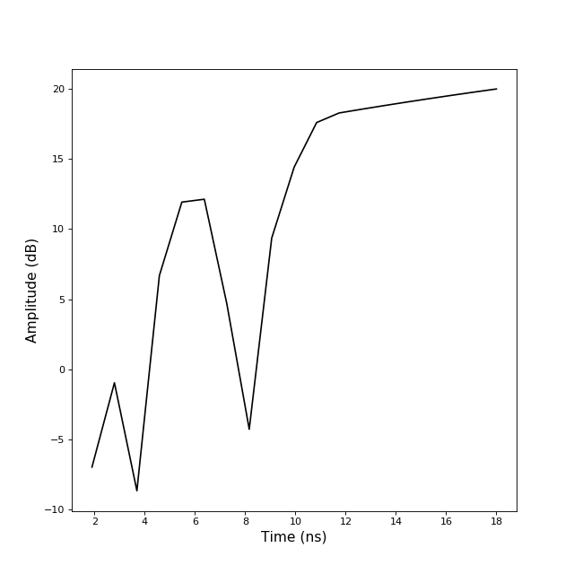
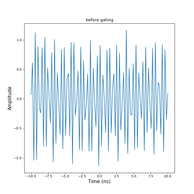
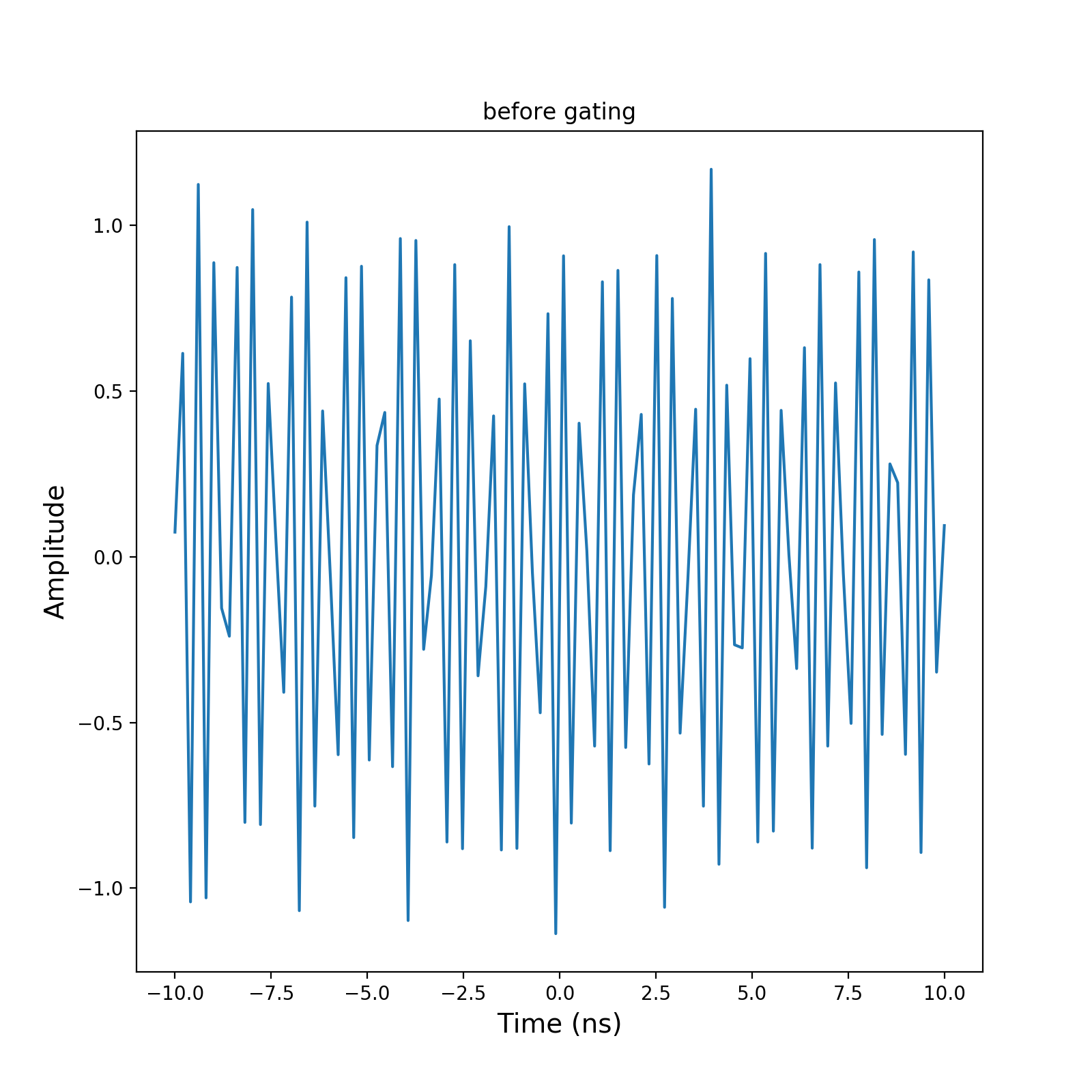
gating(xmin, xmax)

gating between xmin and xmax

xmin : float xmax : float

nothing self is modified

>>> import numpy as np
>>> import matplotlib.pyplot as plt
>>> from pylayers.signal.bsignal import *
>>> x = np.linspace(-10,10,100)
>>> y = np.sin(2*np.pi*12*x)+np.random.normal(0,0.1,len(x))
>>> s = TUsignal(x,y)
>>> fig,ax = s.plot(typ=['v'])
>>> txt1 = plt.title('before gating')
>>> plt.show()

(Source code, png, hires.png, pdf)

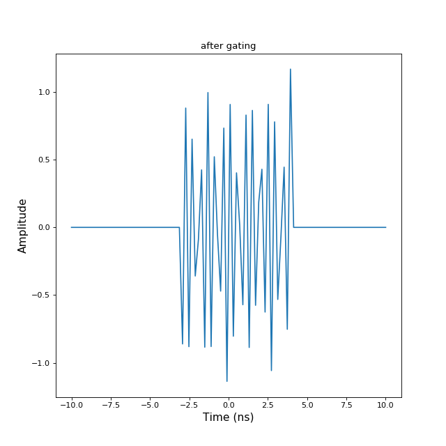
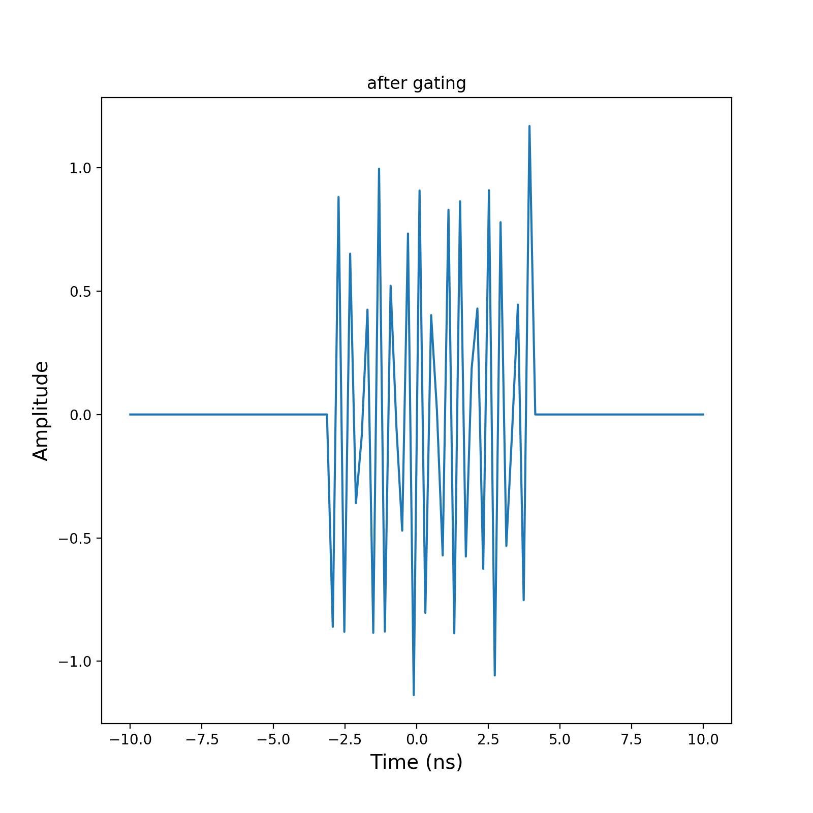
>>> s.gating(-3,4)
>>> fig,ax=s.plot(typ=['v'])
>>> txt2 = plt.title('after gating')
>>> plt.show()

(png, hires.png, pdf)

When a gating is applied the removed information is lost

imshow(**kwargs)

imshow of y matrix

interpolation : string

‘none’|’nearest’|’bilinear’

cmap : colormap

plt.cm.jet

aspect : string

‘auto’ (default) ,’equal’,’scalar’

function : string

{‘imshow’|’pcolormesh’}

typ : string

‘l20’,’l10’

vmin : min value vmax : max value sax : list

select axe

bindex

>>> f = np.arange(100)
>>> y = np.random.randn(50,100)+1j*np.random.randn(50,100)
>>> F = FUsignal(f,y)

len()

returm length of x axis

load(filename)

load a Bsignal from a Matlab File

filename : string

Bsignal.save

max()

max value of the signal (module if complex)

mean()

mean value of the signal

min()

min value of the signal (module if complex)

plot(**kwargs)

plot signal Bsignal

iy : index of the waveform to plot (-1 = all) col : string

default ‘black’

vline : ndarray hline : ndarray unit1 : string

default ‘V’

unit2 : string

default ‘V’

xmin : float xmax : float ax : axes instance or [] dB : boolean

default False

dist : boolean

default False

display : boolean

default True

logx : boolean

defaut False

logy : boolean

default False

fig : figure ax : np.array of axes

pylayers.util.plotutil.mulcplot

save(filename)

save Bsignal in Matlab File Format

filename : string

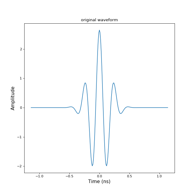
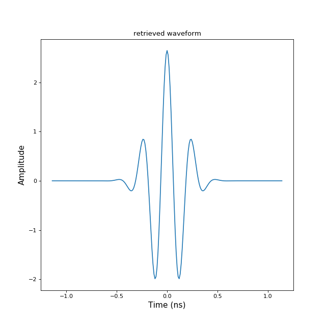
>>> from pylayers.signal.bsignal import *
>>> import matplotlib.pyplot as plt
>>> e = TUsignal()
>>> e.EnImpulse(feGHz=100)
>>> fig,ax = e.plot(typ=['v'])
>>> tit1 = plt.title('original waveform')
>>> e.save('impulse.mat')
>>> del e
>>> h = TUsignal()
>>> h.load('impulse.mat')
>>> fig,ax = h.plot(typ=['v'])
>>> tit2 = plt.title('retrieved waveform')

(Source code)

(png, hires.png, pdf)

(png, hires.png, pdf)

Bsignal.load

setx(x)

setx : set x vector

x : np.array

y is set to a zero vector

Use __set__ instead

sety(fun)

sety : set y vector

fun : function

stem(**kwargs)

stem display

color : string

default ‘b-‘

>>> from pylayers.signal.bsignal import *
>>> import matplotlib.pyplot as plt
>>> si = Bsignal()
>>> si.x= np.arange(100)
>>> si.y= np.arange(100)[None,:]
>>> f,a = si.stem()

(Source code, png, hires.png, pdf)

step(color='b')

plot steps display

color : string

default ‘b-‘

34.2   Usignal Class

34.3   TBsignal Class

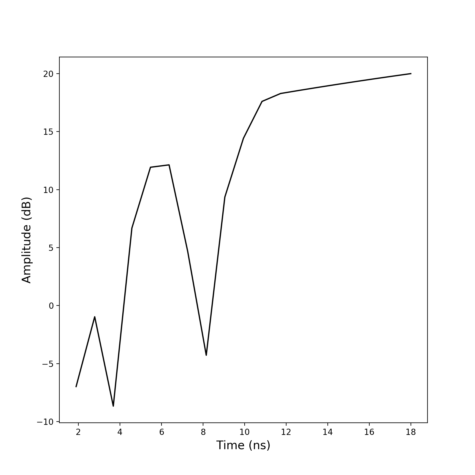
class pylayers.signal.bsignal.TBsignal(x=array([], dtype=float64), y=array([], dtype=float64), label=[])

Based signal in Time domain

b2tu(N)

conversion from TBsignal to TUsignal

N : integer

Number of points

U : TUsignal

This function exploits linear interp1d

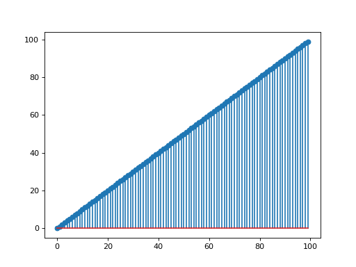
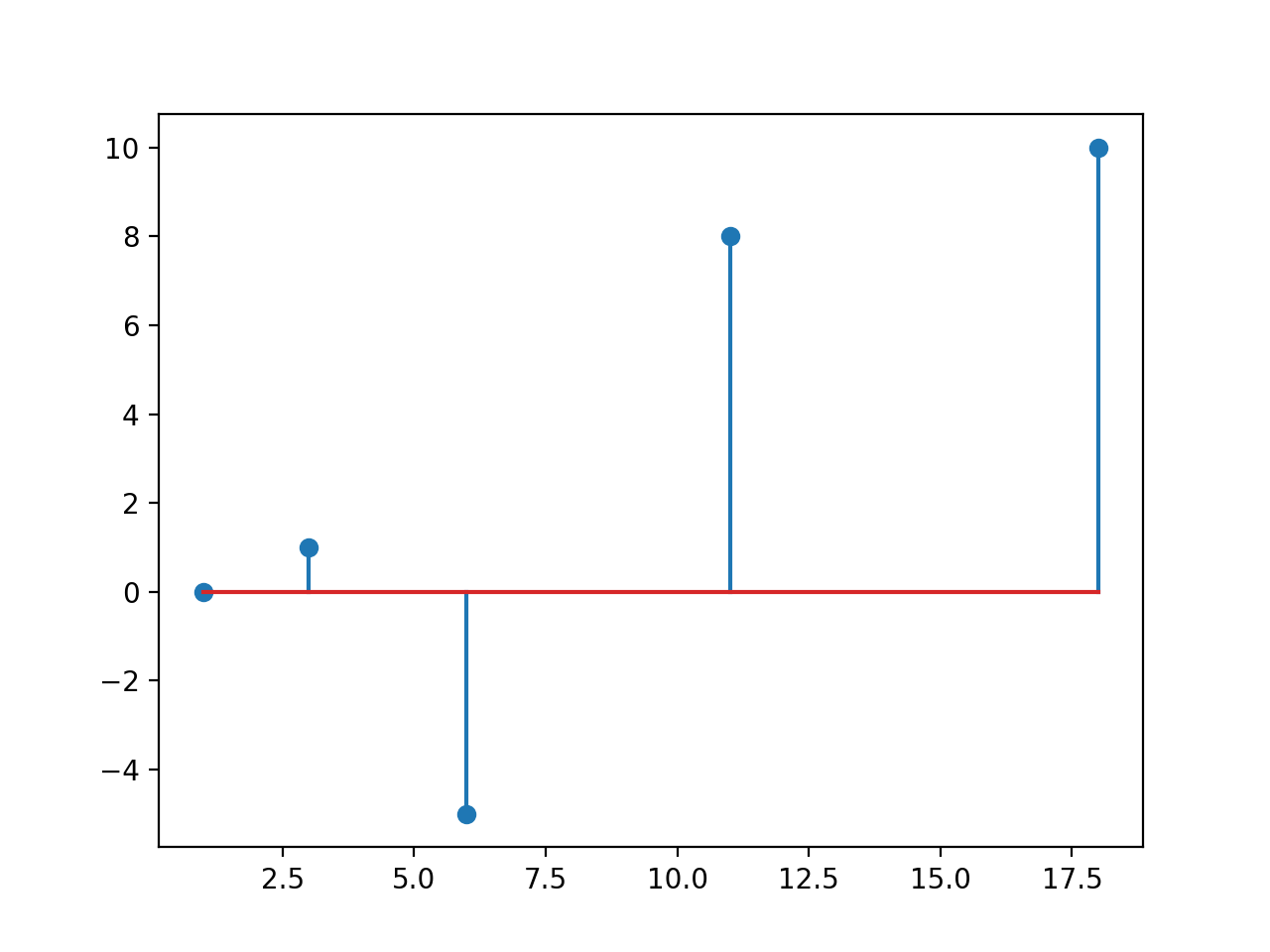
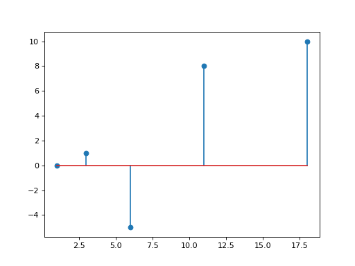
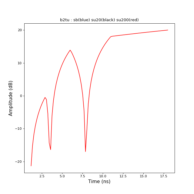
>>> from pylayers.signal.bsignal import *
>>> import matplotlib.pyplot as plt
>>> x = np.array( [ 1, 3 , 6 , 11 , 18])
>>> y = np.array( [ 0,1 ,-5, 8 , 10])
>>> sb = TBsignal(x,y)
>>> su20 = sb.b2tu(20)
>>> su100 = sb.b2tu(100)
>>> fi = plt.figure()
>>> st = sb.stem()
>>> fig,ax = su20.plot(color='k')
>>> fig,ax = su100.plot(color='r')
>>> ti = plt.title('b2tu : sb(blue) su20(black) su200(red)')

(Source code)

(png, hires.png, pdf)

(png, hires.png, pdf)

(png, hires.png, pdf)

(png, hires.png, pdf)

b2tu2(fsGHz, Tobsns)

conversion from TBsignal to TUsignal

N : integer

Number of points

U : TUsignal

This function exploits linear interp1d

>>> from pylayers.signal.bsignal import *
>>> import matplotlib.pyplot as plt
>>> x = np.array( [ 1, 3 , 6 , 11 , 18])
>>> y = np.array( [ 0,1 ,-5, 8 , 10])
>>> sb = TBsignal(x,y)
>>> su20 = sb.b2tu(20)
>>> su100 = sb.b2tu(100)
>>> fi = plt.figure()
>>> st = sb.stem()
>>> fig,ax = su20.plot(color='k')
>>> fig,ax = su100.plot(color='r')
>>> ti = plt.title('b2tu : sb(blue) su20(black) su200(red)')

(Source code)

(png, hires.png, pdf)

(png, hires.png, pdf)

(png, hires.png, pdf)

(png, hires.png, pdf)

integ(Tns, Tsns=50)

integation of alphak tauk of TBsignal

used energy detector for IEEE 802.15.6 standard

Tns : Tsns :

plot(**kwargs)

plot TBsignal

unit1 : actual unit of data unit2 : unit for display dist : boolean xmin : float xmax : float logx : boolean logy :boolean

>>> import numpy as np
>>> from pylayers.signal.bsignal import *
>>> from matplotlib.pylab import *
>>> x = np.array( [ 1, 3 , 6 , 11 , 18])
>>> y = np.array( [ 0,1 ,-5, 8 , 10])
>>> s = Bsignal(x,y)
>>> fi = figure()
>>> fig,ax=s.plot(typ=['v'])
>>> ti = title('TBsignal : plot')
>>> show()

tap(fcGHz, WGHz, Ntap)

Back to baseband

fcGHz : float

center frequency

WGHz : float

bandwidth

Ntap : int

Number of tap

Implement formula (2.52) from D.Tse book page 50

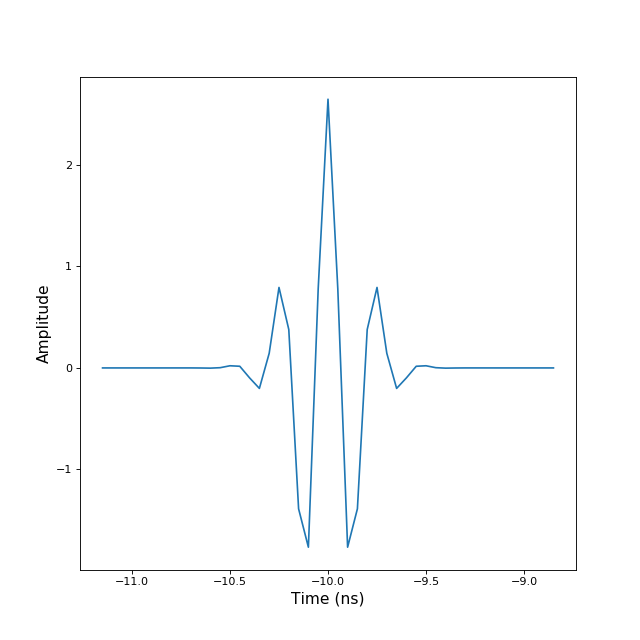
translate(tau)

translate TBsignal signal by tau

tau : float

delay for translation

Once translated original signal and translated signal might not be on the same grid

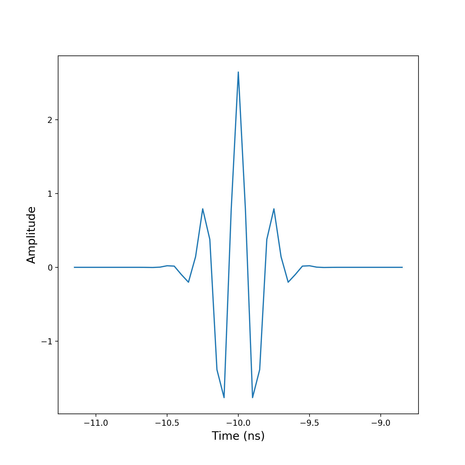
>>> from pylayers.signal.bsignal import *
>>> from matplotlib.pylab import *
>>> ip = TUsignal()
>>> ip.EnImpulse()
>>> ip.translate(-10)
>>> fig,ax=ip.plot(typ=['v'])
>>> show()

(Source code, png, hires.png, pdf)

34.4   TUsignal Class

class pylayers.signal.bsignal.TUsignal(x=array([], dtype=float64), y=array([], dtype=float64), label=[])

Uniform signal in time domain

This class inheritates from TBsignal and Usignal

The signal can either be complex or real

Efirst_loc(nint, E0)

find the Efirst using the mean like

nint E0

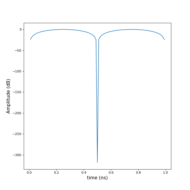
EnImpulse(**kwargs)

Create an energy normalized Gaussian impulse (Usignal)

fcGHz : float WGHz : float threshdB : float feGHz : float

Impulse(**kwargs)

Create a Gaussian impulse (Usignal)

fcGHz : float WGHz : float threshdB : float feGHz : float

MaskImpulse(**kwargs)

MaskImpulse : Create an Energy normalized Gaussian impulse (Usignal)

Yadd_zeros2l(N)

time domain extension on the left with N zeros

N : integer

number of additinal zero values

Yadd_zeros2r

Work only for single y

Yadd_zeros2r(N)

time domain extension on right with N zeros

N : integer

number of additinal zero values

Yadd_zeros2l

align(u2)

align two TUsignal on a same base

returns a list which contains the two aligned signals

It is assume that both signal u1 and u2 share the same dx This function can be improved regarding time granularity

u2 : TUsignal

TUsignal y extended TU signal, x bases are adjusted

>>> import matplotlib.pylab as plt
>>> from pylayers.signal.bsignal import *
>>> i1 = TUsignal()
>>> i2 = TUsignal()
>>> i1.EnImpulse()
>>> i2.EnImpulse()
>>> i2.translate(-10)
>>> i3 = i1.align(i2)
>>> fig,ax=i3.plot(typ=['v'])
>>> plt.show()

(Source code)

convolve(u)

time domain convolution

correlate(s, normalized=True)

correlates with an other TUsignal

s : TUsignal normalized : boolean

default True

The time step dx should be the same

The chosen time reference is the one of the self signal This means that this function can be used to detect events appearing in the self signal by correlating with signal ..math:s, maximum of the correlation function appears in the proper time of the self signal history.

Interpretation of the correlation levels

We assume that s1 is the self signal and s2 is the correlating signal

s1 = a1 * sn(t-tau) where sn is normalized in energy s2 = a2 * sn(t) ” ” ” ” “

the maximum of correlation appears at time tau and its value is

max (s1.correlate(s2,True)) = a1*a2

In the case of the propagation simulation we have

s1 : the time domain UWB received waveform s2 : the corresponding emitted waveform s2,

To determine the ratio a1/a2 or a2/a1 in order to evaluate the propagation Loss L = 20 log10(a2/a1)

This calculus assumes implicitely that the shape of the transmitted signal has not been modified during the propagation, which is a strong hypothesis. This calculus is then a minorant of the received energy.

L = max(s1.correlate(s2,True)/s1.Energy) with a1**2 = sum(s1**s1)*dx

corrgauss(sigma)

Correlate TUsignal with a normalized gaussian of standard deviation sigma

sigma : float

standard deviation of Gaussian

diff()

numerical differentiation TUsignal

the number of points is reduced by one

esd(mode='bilateral')

Calculate the energy spectral density of the U signal

mode : string

‘unilateral’ | ‘bilateral’

FHsignal : if mode == ‘bilateral’ FUsignal : if mode == ‘unilateral’

FHsignal.unrex

fft(shift=False)

forward fast Fourier transform of TUsignal

shift : boolean

default False

This fft is a scaled fft and takes into account the value of the sampling period.

FHsignal

>>> from pylayers.signal.bsignal import *
>>> e = TUsignal()
>>> e.EnImpulse()
>>> E = e.fft()

fftsh()

returns an FHsignal

This fft is a scaled fft and takes into account the value of the sampling period.

FHsignal : Frequency signal with enforced Hermitian symetry

filter(order=4, wp=0.3, ws=0.4, ftype='butter')

TUsignal filtering

order : int wp : float ws : float ftype : string

O : Output filtered TUsignal

ft()

return the associated FUsignal

ftshift()

return the associated FUsignal

H : FUsignal

pylayers.signal.bsignal.TUsignal.fftsh pylayers.signal.waveform.ip_generic

info()

display information about TUsignal

psd(Tpns=100, R=50, periodic=True)

calculate TUsignal power spectral density

R : Resistance (default 50 Ohms) Tpns : real

PRP (default 100 ns)

Note

If time is in ns the resulting PSD is expressed in dBm/MHz (~10-9)

shift(tau)

shift the Usignal by tau (expressed in the same unit as Bsignal.x)

This method uses fft and ifft to produce a shift which is not necessarily a multiple of the time step dx.

tau : float

showpsd(fig=[], ax=[], display=True, PRPns=100)

show psd

fig ax display

pylayers.signal.bsignal.TUsignal.psd pylayers.signal.bsignal.Usignal.zlr

34.5   FBsignal Class

class pylayers.signal.bsignal.FBsignal(x=array([], dtype=float64), y=array([], dtype=float64), label=[])

FBsignal : Base signal in Frequency domain

plot : plot modulus and phase plotri : plot real part and imaginary part plotdB : plot modulus in dB

plot(**kwargs)

plot FBsignal

phase : boolean

default True

dB : boolean

default True

iy : index of y value to be displayed typ : string

[‘l10’,’m,’l20’,’d’,’r’,’du’,’ru’]

xlabels ylabels

>>> from pylayers.signal.bsignal import *
>>> from numpy import *
>>> from scipy import *
>>> S = FBsignal()
>>> S.x = arange(100)
>>> S.y = cos(2*pi*S.x)+1j*sin(3*pi*S.x+pi/3)
>>> fig,ax = S.plot()
>>> plt.show()

Bsignal.plot pylayers.util.plotutil.mulcplot

plotdB(mask=False, n=2, phase=True)

usage : plotdB()

mask : n : phase :

plotri(nb=-1)

plot real and imaginary part

nb : int

stem(color='b-')

stem plot

color : string

34.6   FUsignal Class

class pylayers.signal.bsignal.FUsignal(x=array([], dtype=float64), y=array([], dtype=float64), label=[])

FUsignal : Uniform signal in Frequency Domain

x : nd.array((1xN)) y : Complex nd.array((… x N )

symH : force Hermitian symetry –> FHsignal symHz : force Hermitian symetry with zero padding –> FHsignal align : align two FUsignal on a same frequency base enthrsh : Energy thresholding thresh = 99.99 % dBthrsh : dB thresholding thresh = 40dB ift : Inverse Fourier transform resample : resampling with a new base newdf : resampling with a new df zp : zero padding until len(x) = N plotri : plot real part and imaginary part plotdB : plot modulus in dB get : get k th ray window :

applyFriis()

apply Friis factor

The Friis factor is multiplied to y

\[ \begin{align}\begin{aligned}y := \( \frac{-j c}{4 \pi f} \) y\\x is frequency in GHz\end{aligned}\end{align} \]

boolean isFriis is set to True

dBthrsh(threshdB=40)

dBthrsh : dB thresholding of an FUsignal

decimate(N=2)

decimate FUsignal by N Parameters ———- N : int

decimation factor (default 2)

dftresamp(df_new)

non finished

df_new :

energy(axis=-1, Friis=False, mode='mean')

calculate energy along a given axis of the FUsignal

axis : (default 0) Friis : boolean mode : string

mean (default) | center | integ | first | last

>>> ip = TUsignal()
>>> ip.EnImpulse()
>>> En1 = ip.energy()
>>> assert((En1>0.99) & (En1<1.01))

If Friis is true energy is multiplied by

\(\frac{-j*c}{4 pi fGHz}\)

axis = 0 is ray axis

if mode == ‘mean’

\(E=\frac{1}{K} \sum_k |y_k|^2\)

if mode == ‘integ’

\(E=\delta_x \sum_k |y_k|^2\)

if mode == ‘center’

\(E= |y_{K/2}|^2\)

enthrsh(thresh=99.99)

Energy thresholding of an FUsignal

thresh : float

threshold in percentage (default 99.99)

EMH2 : cumul energie H

get(k)

get the kth signal from the FUsignal

k : indes to get

G : FUsignal

ifft(Npt=-1)

Inverse Fourier transform

Npt : int

default -1 (same number as x)

tc : TUsignal

\[x = \textrm{linspace}(0,\frac{1}{\delta f},N)\]

\[y = [0,\mathbb{X}_u^T]\]

ift(Nz=1, ffts=0, beta=0)

Inverse Fourier Transform - returns the associated TUsignal

Nz : Number of zeros (-1) No forcing ffts : 0 (no fftshift 1:fftshift) beta : kaiser window shape

0 : rectangular 5 : similar to a Hamming 6 : similar to a Hanning 8.6 : similar to a blackman

uh :

>>> from pylayers.signal.bsignal import *
>>> e = TUsignal()
>>> e.EnImpulse()
>>> E  = e.fft()
>>> EU = E.unrex()

1 - Force Hermitian symmetry –> FHsignal with or without zero padding 2 - Inverse Fourier transform with or without fftshift

FHsignal.ifft, FUsignal.symH, FUsignal.symHz

iftshift(Nz=1)

Return the associated TUsignal

apply the inverse fftshift operator to come back in time

info()

Display Information about the FUsignal

newdf(df)

resample the FUsignal using phase and module interpolation

df

U : FUsignal

show(**kwargs)

imshow visualization of Modulus and Phase

vmin : vmax : cmap : colormap

symH(parity=0)

enforce Hermitian symetry

parity : integer

0 even 1 odd

V : FHsignal

symHz(Nz, scale='extract')

Force Hermitian symmetry with zero padding

Nz : int

Number of zero above f[-1]

scale : string

default : ‘extract’ | ‘cir’

SH : FHsignal

The signal is rescaled in order to conserve energy

Let denotes the FUsignal as \(mathcal{X}_d\) The Fourier matrix is :math:`left[ matrix{mathbb{1}\

mathbb{W}_d\ mathbb{W}_u}right]`

FHSignal

>>> N     = 11
>>> x     = np.linspace(2,11,N)
>>> y1    = sp.randn(N)+1j*sp.rand(N)
>>> y2    = sp.randn(N)+1j*sp.rand(N)
>>> y1[0] = 0
>>> y2[0] = 0
>>> y     = np.vstack((y1,y2))
>>> S     = FUsignal(x,y)
>>> FH =  S.symHz(10)

tap(**kwargs)

calculates channel taps

fcGHz : float

center frequency GHz

WGHz : float

bandwidth GHz

Ntap : number of taps baseband : boolean

default : True

htapi

[Tse] David Tse, http://www.eecs.berkeley.edu/~dtse/Chapters_PDF/Fundamentals_Wireless_Communication_chapter2.pdf page 26

zp(N)

zero padding until length N

N : int

FUsignal

34.7   FHsignal Class

34.8   Noise Class

class pylayers.signal.bsignal.Noise(ti=0, tf=100, fsGHz=50, PSDdBmpHz=-174, NF=0, R=50, seed=1)

Create noise

eval()

noise evaluation

$$N_0 = 4 times 10^{-21}$$

fgating(fcGHz, WGHz, window='rect')

apply a frequency gating

fcGHz : float WGHz : float window : string

‘rect’

ppsd(mask=True)

plot Power Spectral Density

mask : boolean

True

34.9   Functions

ExpFunc(x, y)	exponential fitting Parameters ———- x : np.array y : np.array
InvFunc(x, z)	inverse fitting
LegFunc(nn, ntrunc, theta, phi)	Compute Legendre functions Ylm(theta,phi)
PowFunc(x, y)	power fitting
cdf(x[, color, label, lw, xlabel, ylabel, logx])	plot the cumulative density function of x
cformat(x, y, **kwargs)	complex format
coldict()	Color dictionary html color
compint(linterval, zmin, zmax[, tol])	get complementary intervals
copy(x)	Shallow copy operation on arbitrary Python objects.
corrcy(a, b)	cyclic matching correlation
correlate(in1, in2[, mode, method])	Cross-correlate two N-dimensional arrays.
createtrxfile(_filename, freq, phi, theta, …)	Create antenna trx file Usage:createtrxfile(filename,freq,phi,theta,Fpr,Fpi,Ftr,Fti)
cshift(l, offset)	ndarray circular shift Parameters ———- l : ndarray offset : int
cspline1d(signal[, lamb])	Compute cubic spline coefficients for rank-1 array.
cspline1d_eval(cj, newx[, dx, x0])	Evaluate a spline at the new set of points.
cylinder(fig, pa, pb, R)	plot a cylinder
deepcopy(x[, memo, _nil])	Deep copy operation on arbitrary Python objects.
delay(p1, p2)	calculate delay in ns between 2 points
dimcmp(ar1, ar2)	compare shape of arrays
displot(pt, ph[, arrow])	discontinuous plot
encodmtlb(lin)	encode python list of string in Matlab format
extract_block_diag(A, M[, k])	Extracts blocks of size M from the kth diagonal of square matrix A, whose size must be a multiple of M.
fill_block_diag(A, blocks, M[, k])	fill A with blocks of size M from the kth diagonal
fill_block_diagMDA(A, blocks, M[, k])	fill A with blocks of size M from the kth diagonal
firwin(numtaps, cutoff[, width, window, …])	FIR filter design using the window method.
foo(var1, var2[, long_var_name])	A one-line summary that does not use variable names or the function name.
getdir(longname)	get directory of a long name
getlong(shortname, directory)	get a long name
getshort(longname)	get a short name
iirdesign(wp, ws, gpass, gstop[, analog, …])	Complete IIR digital and analog filter design.
iirfilter(N, Wn[, rp, rs, btype, analog, …])	IIR digital and analog filter design given order and critical points.
in_ipynb()	check if program is run in ipython notebook
ininter(ar, val1, val2)	in interval
lfilter(b, a, x[, axis, zi])	Filter data along one-dimension with an IIR or FIR filter.
lt2idic(lt)	convert list of tuple to dictionary
mulcplot(x, y, **kwargs)	handling multiple complex variable plots
nbint(a)	calculate the number of distinct contiguous sets in a sequence of integer
npextract(y, s)	access a numpy MDA while keeping number of axis
pol3D(fig, rho, theta, phi[, sf, shade, title])	polar 3D surface plot
polycol(lpoly[, var])	plot a collection of polygon
printout(text[, colour])
randcol(Nc)	get random color
rectplot(x, xpos[, ylim])	plot rectangles on an axis
rgb(valex[, out])	convert a hexadecimal color into a (r,g,b) array >>> import pylayers.util.pyutil as pyu >>> coldic = pyu.coldict() >>> val = rgb(coldic[‘gold’],’float’)
rotate_line(A, B, theta)	rotation of a line [AB] of an angle theta with A fixed
shadow(data, ax)	data : np.array 0 or 1 ax : matplotlib.axes
shp(arr)	return dimension of an array
sqrte(z)	Evanescent SQRT for waves problems
test()
timestamp(now)
tstincl(ar1, ar2)	test wheteher ar1 interval is included in interval ar2
untie(a, b)	Parameters ———- a : np.array b : np.array
unzipd(path, zipfilename)	unzip a zipfile to a folder
unzipf(path, filepath, zipfilename)	unzip a file from zipfile to a folder
writeDetails(t[, description, location])	write MeasurementsDetails.txt
writemeca(ID, time, p, v, a)	write mecanic information into text file: output/TruePosition.txt output/UWBSensorMeasurements.txt
writenet(net, t)	write network information into text file: netsave/ZIGLinkMeasurements.txt netsave/UWBLinkMeasurements.txt
writenode(agent)	write Nodes.txt
zipd(path, zipfilename)	add a folder to a zipfile

34.10   Classes

Axes3D(fig[, rect])	3D axes object.
Bsignal([x, dtype, y, dtype, label])	Signal with an embedded time base
Error
FBsignal([x, dtype, y, dtype, label])	FBsignal : Base signal in Frequency domain
FHsignal([x, dtype, y, dtype, label])	FHsignal : Hermitian uniform signal in Frequency domain
FUsignal([x, dtype, y, dtype, label])	FUsignal : Uniform signal in Frequency Domain
Noise([ti, tf, fsGHz, PSDdBmpHz, NF, R, seed])	Create noise
PolyCollection(verts[, sizes, closed])
PyLayers	Generic PyLayers Meta Class
TBsignal([x, dtype, y, dtype, label])	Based signal in Time domain
TUsignal([x, dtype, y, dtype, label])	Uniform signal in time domain
Usignal([x, dtype, y, dtype, label])	Signal with an embedded uniform Base

34.11   Class Inheritance Diagram

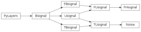
35   pylayers.signal.standard Module

35.1   Classes

AP(**kwargs)	Access Point
Band(**kwargs)	A Band is a structured portion of the spectrum
Channel(fcghz, bmhz[, gmhz])	a radio channel abstraction
PyLayers	Generic PyLayers Meta Class
Wstandard([stdname, _filejson])	Wireless standard class

35.2   Class Inheritance Diagram

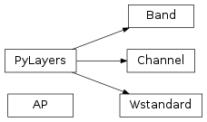
36   pylayers.signal.device Module

This module describes the radio devices to be used for electromagentic simulations

36.1   Device Class

Device.__init__([devname, ID, owner, typ])

init of Device class

36.2   Functions

devicels()

list available devices in project directory

36.3   Classes

Antenna([typ])	Attributes ———-
Device([devname, ID, owner, typ])	Device Class
PyLayers	Generic PyLayers Meta Class
VTKDataSource	This source manages a VTK dataset given to it.
Wstandard([stdname, _filejson])	Wireless standard class

36.4   Class Inheritance Diagram

37   pylayers.signal.DF Module

37.1   DF Class

This class implements a LTI digital filter

class pylayers.signal.DF.DF(b=array([1]), a=array([1]))

Digital Filter Class

a : array

transfer function coefficients denominator

b : array

transfer function coefficients numerator

p : array dtype=complex

transfer function poles

z : array dtype=complex

transfer function zeros

filter : filter a signal freqz : Display transfer function ellip_bp : elliptic bandpath filter remez : FIR design

butter(order=5, w=0.25, typ='low')

Butterwoth digital filter design

order : int

filter order

w : array_like

a scalar or length-2 sequence (relative frequency 0<1 fN <=> 1)

typ : string

‘lowpass’ | ‘highpass’ | ‘bandpass’ | ‘bandstop’

>>> from pylayers.signal.DF import *
>>> flt = DF()
>>> flt.butter(order=3,w=0.25,typ='low')
>>> flt.freqz()

ellip_bp(wp, ws, gpass=0.5, gstop=20)

Elliptic Bandpath filter

wp : ws : gpass gstop :

iirdesign

factorize()

factorize the filter into a minimal phase and maximal phase

(Fmin,Fmax) : tuple of filter

Fmin : minimal phase filter Fmax : maximal phase filter

filter(s, causal=True)

filter s

s : np.array |TUsignal

input signal

y : np.array | TUsignal

output signal

>>> import matplotlib.pyplot as plt
>>> df = DF(b=np.array([1,1],a=np.array([1,-1]))
>>> N = 100
>>> s = np.zeros(N)
>>> s[0] = 1
>>> y = df.filter(s)
>>> plt.stem(np.arange(N),x)
>>> plt.stem(np.arange(N),y)
>>> plt.show()

(Source code)

flipc()

flip coefficient

This is equivalent to the transformation

z -> 1/z

freqz(**kwargs)

freqz : evaluation of filter transfer function

The function evaluates an FUsignal

display : boolean

True

fsGHz : float

if set to 0 (relative frequency)

ir(N=100, show=False)

returns impulse response

ir : np.array

impulse response

match()

return a match filter

DF :

if $$H(z)=\frac{1+b_1z^1+…+b_Nz^{-N}}{1+a_1z^1+…+a_Mz^{-M}}$$

it returns

$$H_m(z)=\frac{b_N+b_{N-1}z^1+…+z^{-N}}{1+a_1z^1+…+a_Mz^{-M}}$$

remez(numtaps=401, bands=(0, 0.1, 0.11, 0.2, 0.21, 0.5), desired=(0.0001, 1, 0.0001))

FIR design Remez algorithm

numtaps : int bands : tuple of N floats desired : tuple of N/2 floats

flt.remez(numtaps=401,bands=(0,0.1,0.11,0.2,0.21,0.5),desired=(0.0001,1,0.0001)):

numtaps = 401 bands = (0,0.1,0.11,0.2,0.21,0.5) desired = (0.0001,1,0.0001))

flt.remez( numtaps , bands , desired)

simplify(tol=1e-16)

simplify transfer function

tol : float

tolerance for simplification

wnxcorr(**kwargs)

filtered noise output autocorrelation

var : float

input noise variance (default = 1)

zplane(title='', fontsize=18)

Display filter in the complex plane

37.2   Classes

DF([b, a])	Digital Filter Class
PyLayers	Generic PyLayers Meta Class

37.3   Class Inheritance Diagram

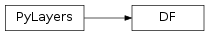
38   pylayers.signal.waveform Module

38.1   Classes

Waveform(**kwargs)

Attributes ———-

38.2   Class Inheritance Diagram

39   pylayers.mobility.agent Module

39.1   Agent Class

class pylayers.mobility.agent.Agent(**args)

Class Agent

args ID name typ net epwr gcom sim wstd sens dcond meca : transit.Person net : pylayers.network.Network sim : PN : rxt rxr

39.2   Classes

Agent(**args)	Class Agent
Containment	Class Containment
Gcom(net, sim)	Communication graph
InterpenetrationConstraint	Class InterpenetrationConstaint
Layout([arg])	Handling Layout
Localization(**args)	Handle localization engine of agents
Network([owner, EMS, PN])	Network class
Node(**kwargs)	Class Node
PLocalization([loc, tx, loc_updt_time, sim])
Person([ID, interval, roomId, L, net, wld, …])	Person Process
RX(**args)	RX process
Seek	class Seek
Separation	Class Separation
TX(**args)	TX process ( not used for now) Each agent use the TX process for querying LDP/information/message passing data to other agent
vec3(*args)	Three-dimensional vector.

39.3   Class Inheritance Diagram

40   pylayers.mobility.ban.body Module

40.1   Body Class

This class implements the body model

class pylayers.mobility.ban.body.Body(_filebody='John.ini', _filemocap=[], _filewear=[], traj=[], unit='cm', loop=True, centered=True, multi_subject_mocap=False, color='white')

Class to manage a Body model

ncyl : number of cylinder sl : d : topos : vtopos :

load center posvel loadC3D settopos setccs setdcs geomfile plot3d movie cylinder_basis_k cyl_antenna

anim()

animate body

>>> from pylayers.mobility.trajectory import *
>>> from pylayers.mobility.ban.body import *
>>> from pylayers.gis.layout import *
>>> T=Trajectories()
>>> T.loadh5()
>>> L=Layout(T.Lfilename)
>>> B = Body()
>>> B.settopos(T[0],t=0,cs=True) 
>>> L._show3()
>>> B.anim(B)

animc3d()

animate c3d file

>>> from pylayers.mobility.trajectory import *
>>> from pylayers.mobility.ban.body import *
>>> B = Body()
>>> B.animc3d(B)

body_link(topos=True, frameId=0)

body link

topos : boolean

default True

frameId : int

used in case topos == False. Indicates the frame Id.

link_vis : np.array (,nlinks)

number of intersected cylinder on the link

links is a list of couple of strings inticating the different links between devices.

c3d2traj()

convert c3d file to trajectory

ccsfromc3d(config)

Create ccs from C3D file

config : dictionnary

center(force=False)

centering the body

self.pg : center of gravity self.vg : velocity self.d : set of centered frames self.smocap : integrated distance self.vmocap : averaged velocity

The center method creates a centered version of the motion capture data stored in self.d It also calculates : self.smocap : total distance along trajectory self.vmocap : averaged speed along trajectory

Here only the projection of the body centroid in the plan 0xy is calculated

chronophoto(**kwargs)

chronophotography of the body movement

(a.k.a. position as a function of time)

tstart : float

starting time in second

tend : float

ending time in second,

tstep : float

time step between tstart and tend

sstep : float

spatial step (distance between 2 instant)

planes : list

list of planes to be displayed [‘xz’,’xy’,’yz’]

dev : bool

show devices

dev : bool

show devices ids

http://en.wikipedia.org/wiki/Chronophotography

cyl_antenna(cylinderId, l, alpha, frameId=0)

cylinder antenna

cylinderId : int index of cylinder l : distance from origin of cylider alpha : angle from reference direction frameId : frameId

cylfromc3d(centered=False)

Create cylinders from C3D file

centered : boolean

False

cylinder_basis_k(frameId)

cylinder basis k

frameId : int

dpdf(tr=[], tunit='ns', poffset=False)

device position dataframe return a dataframe with body and devices positions along the self.traj

tr : ndarray

timerange

cdf: pd.DataFrame

complete device data frame

>>> from pylayers.mobility.ban.body import *
>>> T = tr.Trajectories()
>>> T.loadh5()
>>> B=Body(traj=T[0])
>>> cdf = B.dpdf()

export_csv(unit='mm', df=[], _filename='default.csv', col=['dev_id', 'dev_x', 'dev_y', 'dev_z', 'timestamp'], **kwargs)

geomfile(**kwargs)

create a geomview file from a body configuration

iframe : int frame id (useless if topos==True) verbose : boolean topos : boolean frame id or topos wire : boolean body as a wire or cylinder ccs : boolean display cylinder coordinate system cacs : boolean display cylinder antenna coordinate system acs : boolean display antenna coordinate system struc : boolean displat structure layout tag : string filestruc : string name of the Layout

This function creates either a 3d representation of the frame iframe or if topos==True a representation of the current topos.

getdevT(id=-1, t=[], frameId=[])

get device orientation

id : str | list

device id.

frameId : int

frameid

t : float

time

device orientation

getdevp(id=-1)

get device position

id : str | list

device id.

frameId : int

frameid

t : float

time

device position

init_traj()

create trajectory object from given trajectory or mocap

intersectBody(A, B, topos=True, frameId=0, cyl=[])

intersect Body

A : np.array (3,) B : np.array (3,) topos : boolean frameId : 0 cyl : list

exclusion list

intersect : np.array (,ncyl)

O : AB not intersected by cylinder 1 : AB intersected by cylinder

intersectBody3(A, B, topos=True, frameId=0)

intersect body new version

A B topos frameId cyl

intersect : np.array (,ncyl)

O : AB not intersected by cylinder 1 : AB intersected by cylinder

load(_filebody='John.ini', _filemocap=[], unit=[], _filewear=[])

load a body ini file

_filebody : body short filename

A body .ini file contains 4 sections

• section [nodes]

Node number = Node name + section [cylinder] CylinderId = {‘t’:tail node number, ‘h’:head node number , ‘r’: cylinder’ radius} + section [wearable] + section [mocap]

loadC3D(filename='07_01.c3d', nframes=-1, unit='cm')

load nframes of motion capture C3D file

filename : string

file name

nframes : int

number of frames

unit : str (mm|cm|mm

unit of c3d file

rot : list [‘x’,’y’,’z’]

swap axes of the c3d file

movie(**kwargs)

creates a geomview movie

lframe : [] verbose : False topos : True wire : True ccs : False dcs : False struc : True traj : [] filestruc:’DLR.off’

Body.geomfile

network()

evaluate network topology and dynamics

This function evaluates distance, velocity and acceleration of the radio network nodes

self.D2 : distances between radio nodes self.V2 : velocities between radio nodes self.A2 : accelerations between radio nodes

plot3d(iframe=0, topos=False, fig=[], ax=[], col='b')

scatter 3d plot

iframe : int topos : boolean fig : ax : col : string

fig,ax

posvel(traj, t)

calculate position and velocity

traj : Tajectory DataFrame

nx3

t : float

trajectory time for evaluation of topos

kf : frame integer index kt : trajectory integer index vsn : normalized speed vector along motion capture trajectory (source) wsn : planar vector orthogonal to vsn vtn : normalized speed vector along motion trajectory (target) wtn : planar vector orthogonal to wtn

This funtion takes as argument a trajectory which is a panda dataframe and a time value in the time scale of the trajectory.

t value should of course be in the interval between trajecroty extremal times tmin and tmax.

smax is the maximum distance covered in the whole motion capture sequence.

sk is the distance covered from the begining of the trajectory until the trajectory time t.

The ratio between those 2 distance is rounded to the nearest integer.

:math:`delta = s_k -lceil

rac{s_k}{s_{max}} s_{max}`

k_f is the index of the topos motion capture into the MOCAP

|__________|__________|____________|___________|_____

kf=2

tmin tmax 0 smax sk

rdpdf()

real device position dataframe

setacs()

set antenna coordinate system (acs) from a topos or a set of frames

setccs(frameId=0, topos=False)

set cylinder coordinate system

frameId : int frame id in the mocap dataframe (default 0) topos : boolean default False

self.ccs : ndarray (nc,3,3) Notes —–

There are as many frames as cylinders (body graph edges)

ccs is a MDA (nc x 3 x 3 ) where nc denotes the number of cylinders For each cylinder there is an attached coordinate systems

1st vector 2nd

setcs(topos=True, frameId=0)

set coordinates systems from a topos or a frame id

topos : boolean

default : True

frameId : int

default 0

pylayers.mobility.ban.body.setccs() pylayers.mobility.ban.body.setdcs() pylayers.mobility.ban.body.setacs()

setdcs(topos=True, frameId=0)

set device coordinate system (dcs) from a topos

This method evaluates the set of all dcs. It provides the information necessary for device placement on the body.

If N is the number of antenna an dcs is an MDA of size 3x4xN

topos : boolean

default : True

frameId : int

default 0

self.dcs : dictionnary

>>> import numpy as np
>>> import pylayers.mobility.trajectory as tr
>>> import pylayers.mobility.ban.body as body
>>> import matplotlib.pyplot as plt
>>> time = np.arange(0,10,0.1)
>>> v = 4000/3600.
>>> x = v*time
>>> y = np.zeros(len(time))
>>> traj = tr.Trajectory()
>>> traj.generate()
>>> bc = body.Body()
>>> bc.settopos(traj,2.3,2)
>>> bc.setccs(topos=True)
>>> bc.setdcs()
>>> bc.show(plane='yz',color='b',widthfactor=80)
>>> plt.show()

(Source code)

settopos(traj=[], t=0, cs=True, treadmill=False, p0=array([ 0., 0.]))

translate the body on a time stamped trajectory

traj : ndarray (3,N) t,x,y t : float time for evaluation of topos (seconds) this value should be in the range of the trajectory timestamp

self.topos self.vtopos

>>> import numpy as np
>>> import pylayers.mobility.trajectory as tr
>>> import pylayers.mobility.ban.body as body
>>> import matplotlib.pyplot as plt
>>> time = np.arange(0,10,0.1)
>>> v = 4000/3600.
>>> x = v*time
>>> y = np.zeros(len(time))
>>> traj = tr.Trajectory()
>>> traj.generate()
>>> John = body.Body()
>>> John.settopos(traj,2.3)
>>> fig,ax = John.show(plane='xz',color='b')
>>> plt.title('xz')
>>> plt.show()

(Source code)

topos is the current spatial global position of a body configuration. this method takes as argument a trajectory and a time value t in the trajectory time-scale.

pylayers.util.geomutil.affine

show(**kwargs)

show a 2D plane projection of the body

frameiId : int plane : string

‘yz’ | ‘xz’ | ‘xy’

widthfactor : int topos : boolean

default False

offset = np.array()

1,3

Todo

show3(**kwargs)

create geomfile for frame iframe

iframe : int frame number (useless if topos == True) topos : boolean if True shows the current body topos tag : aditional string for naming file .off (useless if topos==False)

40.2   Cylinder Class

40.3   Functions

ChangeBasis(u0, v0, w0, v1)	change basis
Global_Trajectory(cycle, traj)	global trajectory
dist(A, B)	evaluate the distance between two points A and B
rotation(cycle[, alpha])	rotate a cycle of frames by an angle alpha
translate(cycle, new_origin)	rotate a cycle of frames by an angle alpha

40.4   Classes

Axes3D(fig[, rect])	3D axes object.
Body([_filebody, _filemocap, _filewear, …])	Class to manage a Body model
PyLayers	Generic PyLayers Meta Class

40.5   Class Inheritance Diagram

41   pylayers.measures.cormoran Module

This module handles CORMORAN measurement data

41.1   CorSer Class

class pylayers.measures.cormoran.CorSer(serie=6, day=11, source='CITI', layout=False)

Handle CORMORAN measurement data

Hikob data handling from CORMORAN measurement campaign

11/06/2014

single subject (Bernard and Nicolas)

12/06/2014

several subject (Jihad, Eric , Nicolas)

align(devdf, hkbdf)

DEPRECATED align time of 2 data frames:

the time delta of the second data frame is applyied on the first one (e.g. time for devdf donwsampled by hkb data frame time)

devdf : device dataframe hkbdf : hkbdataframe

devdfc :

aligned copy device dataframe

hkbdfc :

aligned copy hkbdataframe

>>> from pylayers.measures.cormoran import *
>>> S=CorSer(6)
>>> devdf = S.devdf[S.devdf['id']=='HKB:15']
>>> hkbdf = S.hkb['AP1-AnkleLeft']
>>> devdf2,hkbdf2 = S.align(devdf,hkbdf)

animhkb(a, b, interval=10, save=False)

a : node name |number b : node name | number save : bool

animhkbAP(a, AP_list, interval=1, save=False, **kwargs)

a : node name AP_nb=[] save : bool

>>> from pylayers.measures.cormoran import *
>>> S = CorSer(6)
>>> S.animhkbAP('TorsoTopLeft',['AP1','AP2','AP3','AP4'],interval=100,xstart=58,figsize=(20,2))

ant

display device techno, id , id on body, body owner,…

compute_visibility(techno='HKB', square_mda=True, all_links=True)

determine visibility of links for a given techno

techno string

select the given radio technology of the nodes to determine

the visibility matrix

square_mda boolean

select ouput format

True : (device x device x timestamp) False : (link x timestamp)

all_links : bool

compute all links or just those for which data is available

if square_mda = True

intersection : (ndevice x nbdevice x nb_timestamp)

matrice of intersection (1 if link is cut 0 otherwise)

links : (nbdevice)

name of the links

if square_mda = False

intersection : (nblink x nb_timestamp)

matrice of intersection (1 if link is cut 0 otherwise)

links : (nblink x2)

name of the links

>>> from pylayers.measures.cormoran import *
>>> import matplotlib.pyplot as plt
>>> C=CorSer(serie=14,day=12)
>>> inter,links=C.compute_visibility(techno='TCR',square_mda=True)
>>> inter.shape
    (15, 15, 12473)
>>>C.imshowvisibility_i(inter,links)

dev

display device techno, id , id on body, body owner,…

devmapper(a, techno='')

retrieve name of device if input is number

or retrieve number of device if input is name

a : str | int

name |id |bodyid

techno : str

radio techno

a : string

dev name

ia : int

dev number

ba : string

dev refernce in body

subject : string

body owning the device

export_csv(**kwargs)

export to csv devices positions

unit : string (‘mm’|’cm’|’m’),

unit of positions in csv(default mm)

tunit: string

time unit in csv (default ‘ns’)

‘alias’: dict

dictionnary to replace name of the devices into the csv . example : if you want to replace a device id named ‘TCR:34’ to an id = 5, you have to add an entry in the alias dictionnary as : alias.update({‘TCR34’:5})

offset : np.array

apply an offset on positions

a csv file into the folder <PylayersProject>/netsave

getdevp(a, techno='', t='', fId='')

get a device position

a : str | int

name |id

techno : str

radio techno

optional :

t : float | list

given time |[time_start,time_stop]

pa : np.array()

>>> from pylayers.measures.cormoran import *
>>> S=CorSer(serie=34)
>>> a=S.getdevp('AP1','WristLeft')

getlink(a, b, techno='', t='')

get a link value

a : str | int

name |id

b : str | int

name |id

optional :

techno : str

radio techno

t : float | list

given time or [start,stop] time

Pandas Serie

>>> from pylayers.measures.cormoran import *
>>> S=CorSer(serie=34)
>>> S.getlink('AP1','WristLeft')

getlinkd(a, b, techno='', t='')

get the distance for a link between devices

a : str | int

name |id

b : str | int

name |id

optional

techno : str

radio techno

t : float | list

given time or [start,stop] time

dist : np.array()

all distances for all timestamps for the given link

>>> from pylayers.measures.cormoran import *
>>> S = CorSer(serie=6)
>>> d = S.getlinkd('AP1','WristLeft',techno='HKB')

getlinkp(a, b, technoa='', technob='', t='', fId='')

get a link devices positions

a : str | int

name |id

b : str | int

name |id

optional :

technoa : str

radio techno

technob : str

radio techno

t : float | list

given time | [time_start,time_stop]

OR

fId : int

frame id

pa,pb : np.array()

>>> from pylayers.measures.cormoran import *
>>> S=CorSer(serie=34)
>>> a,b=S.getlinkp('AP1','WristLeft')

imshow(time=100, kind='time')

DEPRECATED

kind : string

‘mean’,’std’

imshowvisibility(techno='HKB', t=0, **kwargs)

imshow visibility mda

techno : (HKB|TCR) t : float

time in second

>>> from pylayers.measures.cormoran import *
>>> import matplotlib.pyplot as plt
>>> C=CorSer(serie=6,day=12)
>>> inter,links=C.compute_visibility(techno='TCR',square_mda=True)
>>> i,l=C.imshowvisibility_i(inter,links)

pylayers.measures.CorSer.compute_visibility()

imshowvisibility_i(techno='HKB', t=0, **kwargs)

imshow visibility mda interactive

inter : (nb link x nb link x timestamps) links : (nblinks) time : intial time (s)

>>> from pylayers.measures.cormoran import *
>>> import matplotlib.pyplot as plt
>>> C=CorSer(serie=6,day=12)
>>> inter,links=C.visimda(techno='TCR',square_mda=True)
>>> i,l=C.imshowvisibility_i(inter,links)

lk2nd(lk)

transcode a lk from Id to real name

lk : string

>>> C=Corser(6)
>>> lk = 'HKB:15-HKB:7'
>>> C.lk2nd(lk)

loadlog()

load in self.log the log of the current serie from MeasurementLog.csv

mtlbsave()

Matlab format save

S{day}_{serie}

node_name node_place node_coord

HKB.{linkname}.tr HKB.{linkname}.rssi HKB.{linkname}.td HKB.{linkname}.dist HKB.{linkname}.sh HKB.{linkname}.dsh

TCR.{linkname}.tr HKB.{linkname}.range HKB.{linkname}.td HKB.{linkname}.dist HKB.{linkname}.sh

offset_setter(a='HKB:1', b='HKB:12', techno='', **kwargs)

offset setter

offset_setter_video(a='AP1', b='WristRight', **kwargs)

video offset setter

plot(a, b, techno='', t='', **kwargs)

ploting

a : str | int

name |id

b : str | int

name |id

techno : str (optional)

radio techno

t : float | list (optional)

given time or [start,stop] time

color : color distance : boolean (False)

plot distance instead of value

lin : boolean (False)

display linear value instead of dB

sqrtinv : boolean (False)

apply : “sqrt (1/ dataset)”

xoffset : float (0)

add an offset on x axis

yoffset : float (1|1e3|1e6)

add an offset on y axis

title : boolean (True)

display title

shortlabel : boolean (True)

enable short labelling

fontsize : int (18)

font size

returnlines : boolean

if True return the matplotlib ploted lines

>>> from pylayers.measures.cormoran import *
>>> S = CorSer(6)
>>> f,ax = S.plot('AP1','TorsoTopLeft',techno='HKB')
>>> f,ax = S.pltvisi('AP1','TorsoTopLeft',techno='HKB',fig=f,ax=ax)
>>> #f,ax = S.pltmob(fig=f,ax=ax)
>>> #plt.title('hatch = visibility / gray= mobility')
>>> plt.show()

pltgt(a, b, **kwargs)

plt ground truth

t0 t1 fig ax figsize: tuple linestyle’ inverse :False,

display 1/distance instead of distance

log : boolean

display log for distance intead of distance

gammma’:1.,

mulitplication factor for log : gamma*log(distance) this can be used to fit RSS

mode : string

‘HKB’ | ‘TCR’ | ‘FULL’

visi : boolean,

display visibility

color: string color (‘k’|’m’|’g’),

color to display the visibility area

hatch’: strin hatch type (‘//’)

hatch type to hatch visibility area

fontsize: int

title fontsize

>>> from pylayers.measures.cormoran import *
>>> S=CorSer(6)
>>> S.pltgt('AP1','TorsoTopLeft')

plthkb(a, b, techno='HKB', **kwargs)

plot Hikob devices

DEPRECATED

a : node name |number b : node name | number t0 : start time t1 : stop time

>>> from pylayers.measures.cormoran import *
>>> S = CorSer(6)
>>> f,ax = S.plthkb('AP1','TorsoTopLeft',techno='HKB')
>>> f,ax = S.pltvisi('AP1','TorsoTopLeft',techno='HKB',fig=f,ax=ax)
>>> f,ax = S.pltmob(fig=f,ax=ax)
>>> plt.title('hatch = visibility / gray= mobility')
>>> plt.show()

pltlk(a, b, **kwargs)

plot links

a : string

node a name

b : string

node b name

display: list

techno to be displayed

figsize t0: float

time start

t1 : float

time stop

colhk: plt.color

color of hk curve

colhk2:plt.color

color of hk curve2 ( if recirpocal)

linestylehk:

linestyle hk

coltcr:

color tcr curve

coltcr2:

color of tcr curve2 ( if recirpocal)

linestyletcr:

linestyle tcr

colgt:

color ground truth

inversegt:

invert ground truth

loggt: bool

apply a log10 factor to ground truth

gammagt:

applly a gamma factor to ground truth (if loggt ! )

fontsize:

font size of legend

visi:

display visibility indicator

axs :

list of matplotlib axes

>>> from pylayers.measures.cormoran import *
>>> S=CorSer(6)
>>> S.pltlk('AP1','TorsoTopLeft')

pltmob(**kwargs)

plot mobility

subject: str

subject to display () if ‘’, take the fist one from self.subject)

showvel : boolean

display filtered velocity

velth: float (0.7)

velocity threshold

fo : int (5)

filter order

fw: float (0.02)

0 < fw < 1 (fN <=> 1)

time_offset : int

add time_offset to start later

>>> from pylayers.measures.cormoran import *
>>> S = CorSer(6)
>>> f,ax = S.plthkb('AP1','TorsoTopLeft',techno='HKB')
>>> #f,ax = S.pltvisi('AP1','TorsoTopLeft',techno='HKB',fig=f,ax=ax)
>>> f,ax = S.pltmob(fig=f,ax=ax)
>>> plt.title('hatch = visibility / gray= mobility')
>>> plt.show()

plttcr(a, b, **kwargs)

plot TCR devices

a : node name |number b : node name | number t0 : start time t1 : stop time

pltvisi(a, b, techno='', **kwargs)

plot visibility between link a and b

color:

fill color

hatch:

hatch type

label_pos: (‘top’|’bottom’|’‘)

postion of the label

label_pos_off: float

offset of postion of the label

label_mob: str

prefix of label in mobility

label_stat: str

prefix of label static

>>> from pylayers.measures.cormoran import *
>>> S = CorSer(6)
>>> f,ax = S.plthkb('AP1','TorsoTopLeft',techno='HKB')
>>> f,ax = S.pltvisi('AP1','TorsoTopLeft',techno='HKB',fig=f,ax=ax)
>>> f,ax = S.pltmob(fig=f,ax=ax)
>>> plt.title('hatch = visibility / gray= mobility')
>>> plt.show()

savemat()

save in Matlab Format

showlink(a='AP1', b='BackCenter', technoa='HKB', technob='HKB', **kwargs)

show link configuation for a given frame

a : int

link index

b : int

link index

technoa : string

default ‘HKB’|’TCR’|’BS’

technob

default ‘HKB’|’TCR’|’BS’

phi : float

antenna elevation in rad

showpattern(a, techno='HKB', **kwargs)

show pattern configuation for a given link and frame

a : int

link index

technoa : string

‘HKB’|’TCR’|’BS’

technob

default ‘HKB’|’TCR’|’BS’

phi : float

antenna elevation in rad

fig : ax : t : float phi : float

pi/2

ap : boolean

snapshot(t0=0, offset=15.5, title=True, save=False, fig=[], ax=[], figsize=(10, 10))

single snapshot plot

t0: float offset : float title : boolean save : boolean fig ax figsize : tuple

snapshots(t0=0, t1=10, offset=15.5)

take snapshots

t0 : float t1 : float

visidev(a, b, technoa='HKB', technob='HKB', dsf=10)

get link visibility status

visi : pandas Series

0 : LOS 1 : NLOS

visidev2(a, b, technoa='HKB', technob='HKB', trange=[])

get link visibility status

trange : nd array

time range

visi : pandas Series

0 : LOS 1 : NLOS

vlc()

play video of the associated serie

41.1.1   Notes

Useful members

distdf : distance between radio nodes (122 columns) devdf : device data frame

41.2   Functions

ChangeBasis(u0, v0, w0, v1)	change basis
ExpFunc(x, y)	exponential fitting Parameters ———- x : np.array y : np.array
Global_Trajectory(cycle, traj)	global trajectory
InvFunc(x, z)	inverse fitting
LegFunc(nn, ntrunc, theta, phi)	Compute Legendre functions Ylm(theta,phi)
PolygonPatch(polygon, **kwargs)	Constructs a matplotlib patch from a geometric object
PowFunc(x, y)	power fitting
array(object[, dtype, copy, order, subok, ndmin])	Create an array.
cascaded_union	Returns the union of a sequence of geometries
cdf(x[, color, label, lw, xlabel, ylabel, logx])	plot the cumulative density function of x
coldict()	Color dictionary html color
compint(linterval, zmin, zmax[, tol])	get complementary intervals
cor_log([short])	display cormoran measurement campaign logfile
corrcy(a, b)	cyclic matching correlation
cpu_count	Returns the number of CPUs in the system
createtrxfile(_filename, freq, phi, theta, …)	Create antenna trx file Usage:createtrxfile(filename,freq,phi,theta,Fpr,Fpi,Ftr,Fti)
cshift(l, offset)	ndarray circular shift Parameters ———- l : ndarray offset : int
delay(p1, p2)	calculate delay in ns between 2 points
dimcmp(ar1, ar2)	compare shape of arrays
dist(A, B)	evaluate the distance between two points A and B
dist_sh2rssi(dist, Ssh[, offsetdB])	Parameters ———-
encodmtlb(lin)	encode python list of string in Matlab format
extract_block_diag(A, M[, k])	Extracts blocks of size M from the kth diagonal of square matrix A, whose size must be a multiple of M.
fill_block_diag(A, blocks, M[, k])	fill A with blocks of size M from the kth diagonal
fill_block_diagMDA(A, blocks, M[, k])	fill A with blocks of size M from the kth diagonal
foo(var1, var2[, long_var_name])	A one-line summary that does not use variable names or the function name.
getdir(longname)	get directory of a long name
getlong(shortname, directory)	get a long name
getshort(longname)	get a short name
img_as_ubyte(image[, force_copy])	Convert an image to 8-bit unsigned integer format.
in_ipynb()	check if program is run in ipython notebook
ininter(ar, val1, val2)	in interval
lt2idic(lt)	convert list of tuple to dictionary
make_axes_locatable(axes)
nbint(a)	calculate the number of distinct contiguous sets in a sequence of integer
npextract(y, s)	access a numpy MDA while keeping number of axis
outputGi_func(args)
outputGi_func_test(args)
pbar(verbose, **kwargs)
printout(text[, colour])
randcol(Nc)	get random color
read_gpickle(path)	Read graph object in Python pickle format.
rgb(valex[, out])	convert a hexadecimal color into a (r,g,b) array >>> import pylayers.util.pyutil as pyu >>> coldic = pyu.coldict() >>> val = rgb(coldic[‘gold’],’float’)
rotate_line(A, B, theta)	rotation of a line [AB] of an angle theta with A fixed
rotation(cycle[, alpha])	rotate a cycle of frames by an angle alpha
sqrte(z)	Evanescent SQRT for waves problems
time2npa(lt)	convert pd.datetime.time to numpy array
timestamp(now)
translate(cycle, new_origin)	rotate a cycle of frames by an angle alpha
tstincl(ar1, ar2)	test wheteher ar1 interval is included in interval ar2
untie(a, b)	Parameters ———- a : np.array b : np.array
unzipd(path, zipfilename)	unzip a zipfile to a folder
unzipf(path, filepath, zipfilename)	unzip a file from zipfile to a folder
urlopen(url[, data, timeout, cafile, …])
writeDetails(t[, description, location])	write MeasurementsDetails.txt
write_gpickle(G, path[, protocol])	Write graph in Python pickle format.
writemeca(ID, time, p, v, a)	write mecanic information into text file: output/TruePosition.txt output/UWBSensorMeasurements.txt
writenet(net, t)	write network information into text file: netsave/ZIGLinkMeasurements.txt netsave/UWBLinkMeasurements.txt
writenode(agent)	write Nodes.txt
zipd(path, zipfilename)	add a folder to a zipfile

41.3   Classes

Axes3D(fig[, rect])	3D axes object.
Basemap([llcrnrlon, llcrnrlat, urcrnrlon, …])
Body([_filebody, _filemocap, _filewear, …])	Class to manage a Body model
Button(ax, label[, image, color, hovercolor])	A GUI neutral button.
CheckButtons(ax, labels, actives)	A GUI neutral radio button.
CorSer([serie, day, source, layout])	Handle CORMORAN measurement data
Cursor(ax[, horizOn, vertOn, useblit])	A horizontal and vertical line that spans the axes and moves with the pointer.
DF([b, a])	Digital Filter Class
Layout([arg])	Handling Layout
Pool	alias of pathos.multiprocessing.ProcessPool
PyLayers	Generic PyLayers Meta Class
SelectL(L, fig, ax)	Associates a Layout and a figure
Slider(ax, label, valmin, valmax[, valinit, …])	A slider representing a floating point range.
VTKDataSource	This source manages a VTK dataset given to it.
combinations	combinations(iterable, r) –> combinations object
partial	partial(func, *args, **keywords) - new function with partial application of the given arguments and keywords.
product	product(*iterables, repeat=1) –> product object

41.4   Class Inheritance Diagram